Supported by Dr. Osamu Ogasawara and  . . |
|
Last data update: 2014.03.03 |
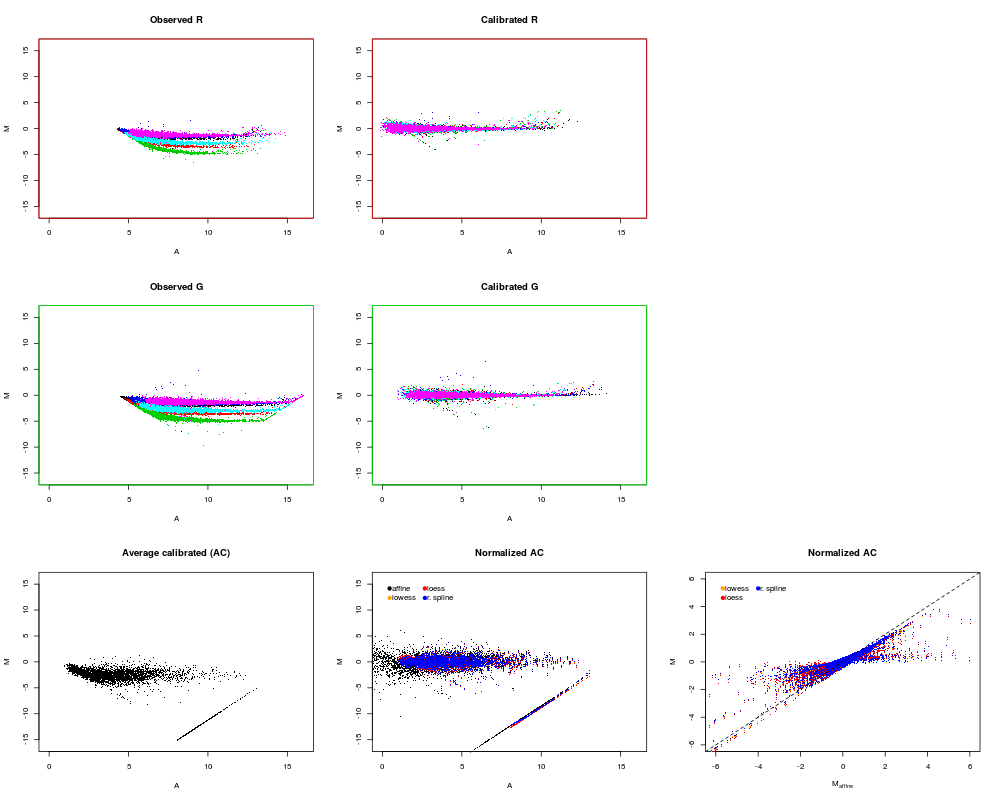
Weighted affine normalization between channels and arraysDescriptionWeighted affine normalization between channels and arrays. This method will remove curvature in the M vs A plots that are due to an affine transformation of the data. In other words, if there are (small or large) biases in the different (red or green) channels, biases that can be equal too, you will get curvature in the M vs A plots and this type of curvature will be removed by this normalization method. Moreover, if you normalize all slides at once, this method will also bring the signals on the same scale such that the log-ratios for different slides are comparable. Thus, do not normalize the scale of the log-ratios between slides afterward. It is recommended to normalize as many slides as possible in one run. The result is that if creating log-ratios between any channels and any slides, they will contain as little curvature as possible. Furthermore, since the relative scale between any two channels on any two slides will be one if one normalizes all slides (and channels) at once it is possible to add or multiply with the same constant to all channels/arrays without introducing curvature. Thus, it is easy to rescale the data afterwards as demonstrated in the example. Usage
## S3 method for class 'matrix'
normalizeAffine(X, weights=NULL, typeOfWeights=c("datapoint"), method="L1",
  constraint=0.05, satSignal=2^16 - 1, ..., .fitOnly=FALSE)
Arguments
DetailsA line is fitted robustly throught the (y_R,y_G) observations using an iterated re-weighted principal component analysis (IWPCA), which minimized the residuals that are orthogonal to the fitted line. Each observation is down-weighted by the inverse of the absolute residuals, i.e. the fit is done in L_1. ValueA NxK Negative, non-positive, and saturated valuesAffine normalization applies equally well to negative values. Thus,
contrary to normalization methods applied to log-ratios, such as curve-fit
normalization methods, affine normalization, will not set these to Data points that are saturated in one or more channels are not used to estimate the normalization function, but they are normalized. Missing valuesThe estimation of the affine normalization function will only be made
based on complete non-saturated observations, i.e. observations that
contains no Weighted normalizationEach data point/observation, that is, each row in RobustnessBy default, the model fit of affine normalization is done in L_1
( For further robustness, downweight outliers such as saturated signals, if possible. We do not use Tukey's biweight function for reasons similar to those
outlined in Using known/previously estimated channel offsetsIf the channel offsets can be assumed to be known, then it is
possible to fit the affine model with no (zero) offset, which
formally is a linear (proportional) model, by specifying
argument Author(s)Henrik Bengtsson References[1] Henrik Bengtsson and Ola Hössjer, Methodological Study of Affine Transformations of Gene Expression Data, Methodological study of affine transformations of gene expression data with proposed robust non-parametric multi-dimensional normalization method, BMC Bioinformatics, 2006, 7:100.
See Also
Examples
pathname <- system.file("data-ex", "PMT-RGData.dat", package="aroma.light")
rg <- read.table(pathname, header=TRUE, sep="\t")
nbrOfScans <- max(rg$slide)

rg <- as.list(rg)
for (field in c("R", "G"))
  rg[[field]] <- matrix(as.double(rg[[field]]), ncol=nbrOfScans)
rg$slide <- rg$spot <- NULL
rg <- as.matrix(as.data.frame(rg))
colnames(rg) <- rep(c("R", "G"), each=nbrOfScans)

layout(matrix(c(1,2,0,3,4,0,5,6,7), ncol=3, byrow=TRUE))

rgC <- rg
for (channel in c("R", "G")) {
  sidx <- which(colnames(rg) == channel)
  channelColor <- switch(channel, R="red", G="green");

  # - - - - - - - - - - - - - - - - - - - - - - - - - - - - - - - -
  # The raw data
  # - - - - - - - - - - - - - - - - - - - - - - - - - - - - - - - -
  plotMvsAPairs(rg[,sidx])
  title(main=paste("Observed", channel))
  box(col=channelColor)

  # - - - - - - - - - - - - - - - - - - - - - - - - - - - - - - - -
  # The calibrated data
  # - - - - - - - - - - - - - - - - - - - - - - - - - - - - - - - -
  rgC[,sidx] <- calibrateMultiscan(rg[,sidx], average=NULL)

  plotMvsAPairs(rgC[,sidx])
  title(main=paste("Calibrated", channel))
  box(col=channelColor)
} # for (channel ...)


# - - - - - - - - - - - - - - - - - - - - - - - - - - - - - - - -
# The average calibrated data
#
# Note how the red signals are weaker than the green. The reason
# for this can be that the scale factor in the green channel is
# greater than in the red channel, but it can also be that there
# is a remaining relative difference in bias between the green
# and the red channel, a bias that precedes the scanning.
# - - - - - - - - - - - - - - - - - - - - - - - - - - - - - - - -
rgCA <- rg
for (channel in c("R", "G")) {
  sidx <- which(colnames(rg) == channel)
  rgCA[,sidx] <- calibrateMultiscan(rg[,sidx])
}

rgCAavg <- matrix(NA, nrow=nrow(rgCA), ncol=2)
colnames(rgCAavg) <- c("R", "G");
for (channel in c("R", "G")) {
  sidx <- which(colnames(rg) == channel)
  rgCAavg[,channel] <- apply(rgCA[,sidx], MARGIN=1, FUN=median, na.rm=TRUE);
}

# Add some "fake" outliers
outliers <- 1:600
rgCAavg[outliers,"G"] <- 50000;

plotMvsA(rgCAavg)
title(main="Average calibrated (AC)")

# - - - - - - - - - - - - - - - - - - - - - - - - - - - - - - - -
# Normalize data
# - - - - - - - - - - - - - - - - - - - - - - - - - - - - - - - -
# Weight-down outliers when normalizing
weights <- rep(1, nrow(rgCAavg));
weights[outliers] <- 0.001;

# Affine normalization of channels
rgCANa <- normalizeAffine(rgCAavg, weights=weights)
# It is always ok to rescale the affine normalized data if its
# done on (R,G); not on (A,M)! However, this is only needed for
# esthetic purposes.
rgCANa <- rgCANa *2^1.4
plotMvsA(rgCANa)
title(main="Normalized AC")

# Curve-fit (lowess) normalization
rgCANlw <- normalizeLowess(rgCAavg, weights=weights)
plotMvsA(rgCANlw, col="orange", add=TRUE)

# Curve-fit (loess) normalization
rgCANl <- normalizeLoess(rgCAavg, weights=weights)
plotMvsA(rgCANl, col="red", add=TRUE)

# Curve-fit (robust spline) normalization
rgCANrs <- normalizeRobustSpline(rgCAavg, weights=weights)
plotMvsA(rgCANrs, col="blue", add=TRUE)

legend(x=0,y=16, legend=c("affine", "lowess", "loess", "r. spline"), pch=19,
       col=c("black", "orange", "red", "blue"), ncol=2, x.intersp=0.3, bty="n")


plotMvsMPairs(cbind(rgCANa, rgCANlw), col="orange", xlab=expression(M[affine]))
title(main="Normalized AC")
plotMvsMPairs(cbind(rgCANa, rgCANl), col="red", add=TRUE)
plotMvsMPairs(cbind(rgCANa, rgCANrs), col="blue", add=TRUE)
abline(a=0, b=1, lty=2)
legend(x=-6,y=6, legend=c("lowess", "loess", "r. spline"), pch=19,
       col=c("orange", "red", "blue"), ncol=2, x.intersp=0.3, bty="n")
Results
R version 3.3.1 (2016-06-21) -- "Bug in Your Hair"
Copyright (C) 2016 The R Foundation for Statistical Computing
Platform: x86_64-pc-linux-gnu (64-bit)

R is free software and comes with ABSOLUTELY NO WARRANTY.
You are welcome to redistribute it under certain conditions.
Type 'license()' or 'licence()' for distribution details.

R is a collaborative project with many contributors.
Type 'contributors()' for more information and
'citation()' on how to cite R or R packages in publications.

Type 'demo()' for some demos, 'help()' for on-line help, or
'help.start()' for an HTML browser interface to help.
Type 'q()' to quit R.

> library(aroma.light)
aroma.light v3.2.0 (2016-01-06) successfully loaded. See ?aroma.light for help.
> png(filename="/home/ddbj/snapshot/RGM3/R_BC/result/aroma.light/normalizeAffine.Rd_%03d_medium.png", width=480, height=480)
> ### Name: normalizeAffine
> ### Title: Weighted affine normalization between channels and arrays
> ### Aliases: normalizeAffine normalizeAffine.matrix
> ### Keywords: methods
>
> ### ** Examples
>
> pathname <- system.file("data-ex", "PMT-RGData.dat", package="aroma.light")
> rg <- read.table(pathname, header=TRUE, sep="\t")
> nbrOfScans <- max(rg$slide)
>
> rg <- as.list(rg)
> for (field in c("R", "G"))
+   rg[[field]] <- matrix(as.double(rg[[field]]), ncol=nbrOfScans)
> rg$slide <- rg$spot <- NULL
> rg <- as.matrix(as.data.frame(rg))
> colnames(rg) <- rep(c("R", "G"), each=nbrOfScans)
>
> layout(matrix(c(1,2,0,3,4,0,5,6,7), ncol=3, byrow=TRUE))
>
> rgC <- rg
> for (channel in c("R", "G")) {
+   sidx <- which(colnames(rg) == channel)
+   channelColor <- switch(channel, R="red", G="green");
+
+   # - - - - - - - - - - - - - - - - - - - - - - - - - - - - - - - -
+   # The raw data
+   # - - - - - - - - - - - - - - - - - - - - - - - - - - - - - - - -
+   plotMvsAPairs(rg[,sidx])
+   title(main=paste("Observed", channel))
+   box(col=channelColor)
+
+   # - - - - - - - - - - - - - - - - - - - - - - - - - - - - - - - -
+   # The calibrated data
+   # - - - - - - - - - - - - - - - - - - - - - - - - - - - - - - - -
+   rgC[,sidx] <- calibrateMultiscan(rg[,sidx], average=NULL)
+
+   plotMvsAPairs(rgC[,sidx])
+   title(main=paste("Calibrated", channel))
+   box(col=channelColor)
+ } # for (channel ...)
>
>
> # - - - - - - - - - - - - - - - - - - - - - - - - - - - - - - - -
> # The average calibrated data
> #
> # Note how the red signals are weaker than the green. The reason
> # for this can be that the scale factor in the green channel is
> # greater than in the red channel, but it can also be that there
> # is a remaining relative difference in bias between the green
> # and the red channel, a bias that precedes the scanning.
> # - - - - - - - - - - - - - - - - - - - - - - - - - - - - - - - -
> rgCA <- rg
> for (channel in c("R", "G")) {
+   sidx <- which(colnames(rg) == channel)
+   rgCA[,sidx] <- calibrateMultiscan(rg[,sidx])
+ }
>
> rgCAavg <- matrix(NA, nrow=nrow(rgCA), ncol=2)
> colnames(rgCAavg) <- c("R", "G");
> for (channel in c("R", "G")) {
+   sidx <- which(colnames(rg) == channel)
+   rgCAavg[,channel] <- apply(rgCA[,sidx], MARGIN=1, FUN=median, na.rm=TRUE);
+ }
>
> # Add some "fake" outliers
> outliers <- 1:600
> rgCAavg[outliers,"G"] <- 50000;
>
> plotMvsA(rgCAavg)
> title(main="Average calibrated (AC)")
>
> # - - - - - - - - - - - - - - - - - - - - - - - - - - - - - - - -
> # Normalize data
> # - - - - - - - - - - - - - - - - - - - - - - - - - - - - - - - -
> # Weight-down outliers when normalizing
> weights <- rep(1, nrow(rgCAavg));
> weights[outliers] <- 0.001;
>
> # Affine normalization of channels
> rgCANa <- normalizeAffine(rgCAavg, weights=weights)
> # It is always ok to rescale the affine normalized data if its
> # done on (R,G); not on (A,M)! However, this is only needed for
> # esthetic purposes.
> rgCANa <- rgCANa *2^1.4
> plotMvsA(rgCANa)
> title(main="Normalized AC")
>
> # Curve-fit (lowess) normalization
> rgCANlw <- normalizeLowess(rgCAavg, weights=weights)
Warning message:
In normalizeCurveFit.matrix(X, method = "lowess", ...) :
  Weights were rounded to {0,1} since 'lowess' normalization supports only zero-one weights.
> plotMvsA(rgCANlw, col="orange", add=TRUE)
>
> # Curve-fit (loess) normalization
> rgCANl <- normalizeLoess(rgCAavg, weights=weights)
> plotMvsA(rgCANl, col="red", add=TRUE)
>
> # Curve-fit (robust spline) normalization
> rgCANrs <- normalizeRobustSpline(rgCAavg, weights=weights)
> plotMvsA(rgCANrs, col="blue", add=TRUE)
>
> legend(x=0,y=16, legend=c("affine", "lowess", "loess", "r. spline"), pch=19,
+        col=c("black", "orange", "red", "blue"), ncol=2, x.intersp=0.3, bty="n")
>
>
> plotMvsMPairs(cbind(rgCANa, rgCANlw), col="orange", xlab=expression(M[affine]))
> title(main="Normalized AC")
> plotMvsMPairs(cbind(rgCANa, rgCANl), col="red", add=TRUE)
> plotMvsMPairs(cbind(rgCANa, rgCANrs), col="blue", add=TRUE)
> abline(a=0, b=1, lty=2)
> legend(x=-6,y=6, legend=c("lowess", "loess", "r. spline"), pch=19,
+        col=c("orange", "red", "blue"), ncol=2, x.intersp=0.3, bty="n")
>
>
>
>
>
>
> dev.off()
null device
          1
>
|