Supported by Dr. Osamu Ogasawara and  . . |
|
Last data update: 2014.03.03 |
Weighted curve-fit normalization between a pair of channelsDescriptionWeighted curve-fit normalization between a pair of channels. This method will estimate a smooth function of the dependency between the log-ratios and the log-intensity of the two channels and then correct the log-ratios (only) in order to remove the dependency. This is method is also known as intensity-dependent or lowess normalization. The curve-fit methods are by nature limited to paired-channel data. There exist at least one method trying to overcome this limitation, namely the cyclic-lowess [1], which applies the paired curve-fit method iteratively over all pairs of channels/arrays. Cyclic-lowess is not implented here. We recommend that affine normalization [2] is used instead of curve-fit normalization. Usage
## S3 method for class 'matrix'
normalizeCurveFit(X, weights=NULL, typeOfWeights=c("datapoint"),
  method=c("loess", "lowess", "spline", "robustSpline"), bandwidth=NULL,
  satSignal=2^16 - 1, ...)
## S3 method for class 'matrix'
normalizeLoess(X, ...)
## S3 method for class 'matrix'
normalizeLowess(X, ...)
## S3 method for class 'matrix'
normalizeSpline(X, ...)
## S3 method for class 'matrix'
normalizeRobustSpline(X, ...)
Arguments
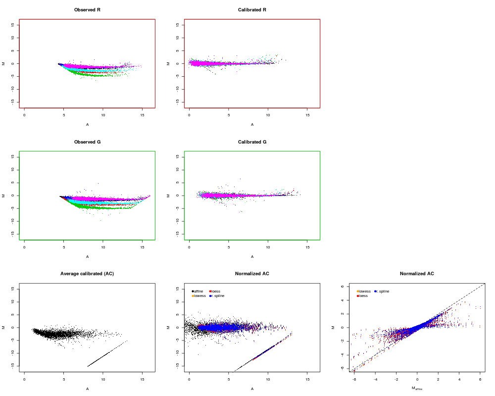
DetailsA smooth function c(A) is fitted throught data in (A,M), where M=log_2(y_2/y_1) and A=1/2*log_2(y_2*y_1). Data is normalized by M <- M - c(A). Loess is by far the slowest method of the four, then lowess, and then robust spline, which iteratively calls the spline method. ValueA Nx2 Negative, non-positive, and saturated valuesNon-positive values are set to not-a-number ( Missing valuesThe estimation of the normalization function will only be made
based on complete non-saturated observations, i.e. observations that
contains no Weighted normalizationEach data point, that is, each row in Note that the lowess and the spline method only support zero-one {0,1} weights. For such methods, all weights that are less than a half are set to zero. Details on loessFor Author(s)Henrik Bengtsson References[1] M. Ã
strand,
Contrast Normalization of Oligonucleotide Arrays,
Journal Computational Biology, 2003, 10, 95-102. See Also
Examples
 pathname <- system.file("data-ex", "PMT-RGData.dat", package="aroma.light")
rg <- read.table(pathname, header=TRUE, sep="\t")
nbrOfScans <- max(rg$slide)

rg <- as.list(rg)
for (field in c("R", "G"))
  rg[[field]] <- matrix(as.double(rg[[field]]), ncol=nbrOfScans)
rg$slide <- rg$spot <- NULL
rg <- as.matrix(as.data.frame(rg))
colnames(rg) <- rep(c("R", "G"), each=nbrOfScans)

layout(matrix(c(1,2,0,3,4,0,5,6,7), ncol=3, byrow=TRUE))

rgC <- rg
for (channel in c("R", "G")) {
  sidx <- which(colnames(rg) == channel)
  channelColor <- switch(channel, R="red", G="green");

  # - - - - - - - - - - - - - - - - - - - - - - - - - - - - - - - -
  # The raw data
  # - - - - - - - - - - - - - - - - - - - - - - - - - - - - - - - -
  plotMvsAPairs(rg[,sidx])
  title(main=paste("Observed", channel))
  box(col=channelColor)

  # - - - - - - - - - - - - - - - - - - - - - - - - - - - - - - - -
  # The calibrated data
  # - - - - - - - - - - - - - - - - - - - - - - - - - - - - - - - -
  rgC[,sidx] <- calibrateMultiscan(rg[,sidx], average=NULL)

  plotMvsAPairs(rgC[,sidx])
  title(main=paste("Calibrated", channel))
  box(col=channelColor)
} # for (channel ...)


# - - - - - - - - - - - - - - - - - - - - - - - - - - - - - - - -
# The average calibrated data
#
# Note how the red signals are weaker than the green. The reason
# for this can be that the scale factor in the green channel is
# greater than in the red channel, but it can also be that there
# is a remaining relative difference in bias between the green
# and the red channel, a bias that precedes the scanning.
# - - - - - - - - - - - - - - - - - - - - - - - - - - - - - - - -
rgCA <- rg
for (channel in c("R", "G")) {
  sidx <- which(colnames(rg) == channel)
  rgCA[,sidx] <- calibrateMultiscan(rg[,sidx])
}

rgCAavg <- matrix(NA, nrow=nrow(rgCA), ncol=2)
colnames(rgCAavg) <- c("R", "G");
for (channel in c("R", "G")) {
  sidx <- which(colnames(rg) == channel)
  rgCAavg[,channel] <- apply(rgCA[,sidx], MARGIN=1, FUN=median, na.rm=TRUE);
}

# Add some "fake" outliers
outliers <- 1:600
rgCAavg[outliers,"G"] <- 50000;

plotMvsA(rgCAavg)
title(main="Average calibrated (AC)")

# - - - - - - - - - - - - - - - - - - - - - - - - - - - - - - - -
# Normalize data
# - - - - - - - - - - - - - - - - - - - - - - - - - - - - - - - -
# Weight-down outliers when normalizing
weights <- rep(1, nrow(rgCAavg));
weights[outliers] <- 0.001;

# Affine normalization of channels
rgCANa <- normalizeAffine(rgCAavg, weights=weights)
# It is always ok to rescale the affine normalized data if its
# done on (R,G); not on (A,M)! However, this is only needed for
# esthetic purposes.
rgCANa <- rgCANa *2^1.4
plotMvsA(rgCANa)
title(main="Normalized AC")

# Curve-fit (lowess) normalization
rgCANlw <- normalizeLowess(rgCAavg, weights=weights)
plotMvsA(rgCANlw, col="orange", add=TRUE)

# Curve-fit (loess) normalization
rgCANl <- normalizeLoess(rgCAavg, weights=weights)
plotMvsA(rgCANl, col="red", add=TRUE)

# Curve-fit (robust spline) normalization
rgCANrs <- normalizeRobustSpline(rgCAavg, weights=weights)
plotMvsA(rgCANrs, col="blue", add=TRUE)

legend(x=0,y=16, legend=c("affine", "lowess", "loess", "r. spline"), pch=19,
       col=c("black", "orange", "red", "blue"), ncol=2, x.intersp=0.3, bty="n")


plotMvsMPairs(cbind(rgCANa, rgCANlw), col="orange", xlab=expression(M[affine]))
title(main="Normalized AC")
plotMvsMPairs(cbind(rgCANa, rgCANl), col="red", add=TRUE)
plotMvsMPairs(cbind(rgCANa, rgCANrs), col="blue", add=TRUE)
abline(a=0, b=1, lty=2)
legend(x=-6,y=6, legend=c("lowess", "loess", "r. spline"), pch=19,
       col=c("orange", "red", "blue"), ncol=2, x.intersp=0.3, bty="n")
Results
R version 3.3.1 (2016-06-21) -- "Bug in Your Hair"
Copyright (C) 2016 The R Foundation for Statistical Computing
Platform: x86_64-pc-linux-gnu (64-bit)

R is free software and comes with ABSOLUTELY NO WARRANTY.
You are welcome to redistribute it under certain conditions.
Type 'license()' or 'licence()' for distribution details.

R is a collaborative project with many contributors.
Type 'contributors()' for more information and
'citation()' on how to cite R or R packages in publications.

Type 'demo()' for some demos, 'help()' for on-line help, or
'help.start()' for an HTML browser interface to help.
Type 'q()' to quit R.

> library(aroma.light)
aroma.light v3.2.0 (2016-01-06) successfully loaded. See ?aroma.light for help.
> png(filename="/home/ddbj/snapshot/RGM3/R_BC/result/aroma.light/normalizeCurveFit.Rd_%03d_medium.png", width=480, height=480)
> ### Name: normalizeCurveFit
> ### Title: Weighted curve-fit normalization between a pair of channels
> ### Aliases: normalizeCurveFit normalizeLoess normalizeLowess
> ###   normalizeSpline normalizeRobustSpline normalizeCurveFit.matrix
> ###   normalizeLoess.matrix normalizeLowess.matrix normalizeSpline.matrix
> ###   normalizeRobustSpline.matrix
> ### Keywords: methods
>
> ### ** Examples
>
>  pathname <- system.file("data-ex", "PMT-RGData.dat", package="aroma.light")
> rg <- read.table(pathname, header=TRUE, sep="\t")
> nbrOfScans <- max(rg$slide)
>
> rg <- as.list(rg)
> for (field in c("R", "G"))
+   rg[[field]] <- matrix(as.double(rg[[field]]), ncol=nbrOfScans)
> rg$slide <- rg$spot <- NULL
> rg <- as.matrix(as.data.frame(rg))
> colnames(rg) <- rep(c("R", "G"), each=nbrOfScans)
>
> layout(matrix(c(1,2,0,3,4,0,5,6,7), ncol=3, byrow=TRUE))
>
> rgC <- rg
> for (channel in c("R", "G")) {
+   sidx <- which(colnames(rg) == channel)
+   channelColor <- switch(channel, R="red", G="green");
+
+   # - - - - - - - - - - - - - - - - - - - - - - - - - - - - - - - -
+   # The raw data
+   # - - - - - - - - - - - - - - - - - - - - - - - - - - - - - - - -
+   plotMvsAPairs(rg[,sidx])
+   title(main=paste("Observed", channel))
+   box(col=channelColor)
+
+   # - - - - - - - - - - - - - - - - - - - - - - - - - - - - - - - -
+   # The calibrated data
+   # - - - - - - - - - - - - - - - - - - - - - - - - - - - - - - - -
+   rgC[,sidx] <- calibrateMultiscan(rg[,sidx], average=NULL)
+
+   plotMvsAPairs(rgC[,sidx])
+   title(main=paste("Calibrated", channel))
+   box(col=channelColor)
+ } # for (channel ...)
>
>
> # - - - - - - - - - - - - - - - - - - - - - - - - - - - - - - - -
> # The average calibrated data
> #
> # Note how the red signals are weaker than the green. The reason
> # for this can be that the scale factor in the green channel is
> # greater than in the red channel, but it can also be that there
> # is a remaining relative difference in bias between the green
> # and the red channel, a bias that precedes the scanning.
> # - - - - - - - - - - - - - - - - - - - - - - - - - - - - - - - -
> rgCA <- rg
> for (channel in c("R", "G")) {
+   sidx <- which(colnames(rg) == channel)
+   rgCA[,sidx] <- calibrateMultiscan(rg[,sidx])
+ }
>
> rgCAavg <- matrix(NA, nrow=nrow(rgCA), ncol=2)
> colnames(rgCAavg) <- c("R", "G");
> for (channel in c("R", "G")) {
+   sidx <- which(colnames(rg) == channel)
+   rgCAavg[,channel] <- apply(rgCA[,sidx], MARGIN=1, FUN=median, na.rm=TRUE);
+ }
>
> # Add some "fake" outliers
> outliers <- 1:600
> rgCAavg[outliers,"G"] <- 50000;
>
> plotMvsA(rgCAavg)
> title(main="Average calibrated (AC)")
>
> # - - - - - - - - - - - - - - - - - - - - - - - - - - - - - - - -
> # Normalize data
> # - - - - - - - - - - - - - - - - - - - - - - - - - - - - - - - -
> # Weight-down outliers when normalizing
> weights <- rep(1, nrow(rgCAavg));
> weights[outliers] <- 0.001;
>
> # Affine normalization of channels
> rgCANa <- normalizeAffine(rgCAavg, weights=weights)
> # It is always ok to rescale the affine normalized data if its
> # done on (R,G); not on (A,M)! However, this is only needed for
> # esthetic purposes.
> rgCANa <- rgCANa *2^1.4
> plotMvsA(rgCANa)
> title(main="Normalized AC")
>
> # Curve-fit (lowess) normalization
> rgCANlw <- normalizeLowess(rgCAavg, weights=weights)
Warning message:
In normalizeCurveFit.matrix(X, method = "lowess", ...) :
  Weights were rounded to {0,1} since 'lowess' normalization supports only zero-one weights.
> plotMvsA(rgCANlw, col="orange", add=TRUE)
>
> # Curve-fit (loess) normalization
> rgCANl <- normalizeLoess(rgCAavg, weights=weights)
> plotMvsA(rgCANl, col="red", add=TRUE)
>
> # Curve-fit (robust spline) normalization
> rgCANrs <- normalizeRobustSpline(rgCAavg, weights=weights)
> plotMvsA(rgCANrs, col="blue", add=TRUE)
>
> legend(x=0,y=16, legend=c("affine", "lowess", "loess", "r. spline"), pch=19,
+        col=c("black", "orange", "red", "blue"), ncol=2, x.intersp=0.3, bty="n")
>
>
> plotMvsMPairs(cbind(rgCANa, rgCANlw), col="orange", xlab=expression(M[affine]))
> title(main="Normalized AC")
> plotMvsMPairs(cbind(rgCANa, rgCANl), col="red", add=TRUE)
> plotMvsMPairs(cbind(rgCANa, rgCANrs), col="blue", add=TRUE)
> abline(a=0, b=1, lty=2)
> legend(x=-6,y=6, legend=c("lowess", "loess", "r. spline"), pch=19,
+        col=c("orange", "red", "blue"), ncol=2, x.intersp=0.3, bty="n")
>
>
>
>
>
>
>
> dev.off()
null device
          1
>
|