R Graphical Manual

Browse All

Last data update: 2014.03.03

R: Normalizes signals for PCR fragment-length effects

normalizeFragmentLength

R Documentation

Normalizes signals for PCR fragment-length effects

Description

Normalizes signals for PCR fragment-length effects. Some or all signals are used to estimated the normalization function. All signals are normalized.

Usage

## Default S3 method:
normalizeFragmentLength(y, fragmentLengths, targetFcns=NULL, subsetToFit=NULL,
  onMissing=c("ignore", "median"), .isLogged=TRUE, ..., .returnFit=FALSE)

Arguments

`y`	A `numeric` `vector` of length K of signals to be normalized across E enzymes.
`fragmentLengths`	An `integer` KxE `matrix` of fragment lengths.
`targetFcns`	An optional `list` of E `function`s; one per enzyme. If `NULL`, the data is normalized to have constant fragment-length effects (all equal to zero on the log-scale).
`subsetToFit`	The subset of data points used to fit the normalization function. If `NULL`, all data points are considered.
`onMissing`	Specifies how data points for which there is no fragment length is normalized. If `"ignore"`, the values are not modified. If `"median"`, the values are updated to have the same robust average as the other data points.
`.isLogged`	A `logical`.
`...`	Additional arguments passed to `lowess`.
`.returnFit`	A `logical`.

Value

Returns a numeric vector of the normalized signals.

Multi-enzyme normalization

It is assumed that the fragment-length effects from multiple enzymes added (with equal weights) on the intensity scale. The fragment-length effects are fitted for each enzyme separately based on units that are exclusively for that enzyme. If there are no or very such units for an enzyme, the assumptions of the model are not met and the fit will fail with an error. Then, from the above single-enzyme fits the average effect across enzymes is the calculated for each unit that is on multiple enzymes.

Target functions

It is possible to specify custom target function effects for each enzyme via argument targetFcns. This argument has to be a list containing one function per enzyme and ordered in the same order as the enzyme are in the columns of argument fragmentLengths. For instance, if one wish to normalize the signals such that their mean signal as a function of fragment length effect is contantly equal to 2200 (or the intensity scale), the use targetFcns=function(fl, ...) log2(2200) which completely ignores fragment-length argument 'fl' and always returns a constant. If two enzymes are used, then use targetFcns=rep(list(function(fl, ...) log2(2200)), 2).

Note, if targetFcns is NULL, this corresponds to targetFcns=rep(list(function(fl, ...) 0), ncol(fragmentLengths)).

Alternatively, if one wants to only apply minimial corrections to the signals, then one can normalize toward target functions that correspond to the fragment-length effect of the average array.

Author(s)

Henrik Bengtsson

References

[1] H. Bengtsson, R. Irizarry, B. Carvalho, and T. Speed, Estimation and assessment of raw copy numbers at the single locus level, Bioinformatics, 2008.

Examples

  # - - - - - - - - - - - - - - - - - - - - - - - - - - - - - - - - - -
# Example 1: Single-enzyme fragment-length normalization of 6 arrays
# - - - - - - - - - - - - - - - - - - - - - - - - - - - - - - - - - -
# Number samples
I <- 9;

# Number of loci
J <- 1000;

# Fragment lengths
fl <- seq(from=100, to=1000, length.out=J);

# Simulate data points with unknown fragment lengths
hasUnknownFL <- seq(from=1, to=J, by=50);
fl[hasUnknownFL] <- NA;

# Simulate data
y <- matrix(0, nrow=J, ncol=I);
maxY <- 12;
for (kk in 1:I) {
  k <- runif(n=1, min=3, max=5);
  mu <- function(fl) {
    mu <- rep(maxY, length(fl));
    ok <- !is.na(fl);
    mu[ok] <- mu[ok] - fl[ok]^{1/k};
    mu;
  }
  eps <- rnorm(J, mean=0, sd=1);
  y[,kk] <- mu(fl) + eps;
}

# Normalize data (to a zero baseline)
yN <- apply(y, MARGIN=2, FUN=function(y) {
  normalizeFragmentLength(y, fragmentLengths=fl, onMissing="median");
})

# The correction factors
rho <- y-yN;
print(summary(rho));
# The correction for units with unknown fragment lengths
# equals the median correction factor of all other units
print(summary(rho[hasUnknownFL,]));

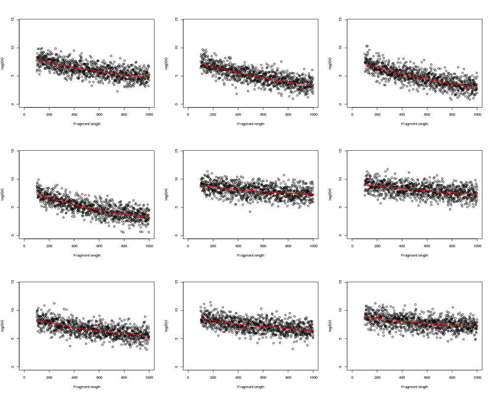
# Plot raw data
layout(matrix(1:9, ncol=3));
xlim <- c(0,max(fl, na.rm=TRUE));
ylim <- c(0,max(y, na.rm=TRUE));
xlab <- "Fragment length";
ylab <- expression(log2(theta));
for (kk in 1:I) {
  plot(fl, y[,kk], xlim=xlim, ylim=ylim, xlab=xlab, ylab=ylab);
  ok <- (is.finite(fl) & is.finite(y[,kk]));
  lines(lowess(fl[ok], y[ok,kk]), col="red", lwd=2);
}

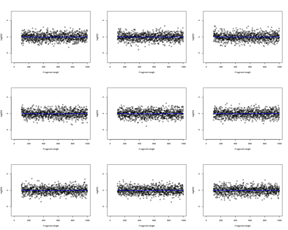
# Plot normalized data
layout(matrix(1:9, ncol=3));
ylim <- c(-1,1)*max(y, na.rm=TRUE)/2;
for (kk in 1:I) {
  plot(fl, yN[,kk], xlim=xlim, ylim=ylim, xlab=xlab, ylab=ylab);
  ok <- (is.finite(fl) & is.finite(y[,kk]));
  lines(lowess(fl[ok], yN[ok,kk]), col="blue", lwd=2);
}


  # - - - - - - - - - - - - - - - - - - - - - - - - - - - - - - - - - -
# Example 2: Two-enzyme fragment-length normalization of 6 arrays
# - - - - - - - - - - - - - - - - - - - - - - - - - - - - - - - - - -
set.seed(0xbeef);

# Number samples
I <- 5;

# Number of loci
J <- 3000;

# Fragment lengths (two enzymes)
fl <- matrix(0, nrow=J, ncol=2);
fl[,1] <- seq(from=100, to=1000, length.out=J);
fl[,2] <- seq(from=1000, to=100, length.out=J);

# Let 1/2 of the units be on both enzymes
fl[seq(from=1, to=J, by=4),1] <- NA;
fl[seq(from=2, to=J, by=4),2] <- NA;

# Let some have unknown fragment lengths
hasUnknownFL <- seq(from=1, to=J, by=15);
fl[hasUnknownFL,] <- NA;

# Sty/Nsp mixing proportions:
rho <- rep(1, I);
rho[1] <- 1/3;  # Less Sty in 1st sample
rho[3] <- 3/2;  # More Sty in 3rd sample


# Simulate data
z <- array(0, dim=c(J,2,I));
maxLog2Theta <- 12;
for (ii in 1:I) {
  # Common effect for both enzymes
  mu <- function(fl) {
    k <- runif(n=1, min=3, max=5);
    mu <- rep(maxLog2Theta, length(fl));
    ok <- is.finite(fl);
    mu[ok] <- mu[ok] - fl[ok]^{1/k};
    mu;
  }

  # Calculate the effect for each data point
  for (ee in 1:2) {
    z[,ee,ii] <- mu(fl[,ee]);
  }

  # Update the Sty/Nsp mixing proportions
  ee <- 2;
  z[,ee,ii] <- rho[ii]*z[,ee,ii];

  # Add random errors
  for (ee in 1:2) {
    eps <- rnorm(J, mean=0, sd=1/sqrt(2));
    z[,ee,ii] <- z[,ee,ii] + eps;
  }
}


hasFl <- is.finite(fl);

unitSets <- list(
  nsp  = which( hasFl[,1] & !hasFl[,2]),
  sty  = which(!hasFl[,1] &  hasFl[,2]),
  both = which( hasFl[,1] &  hasFl[,2]),
  none = which(!hasFl[,1] & !hasFl[,2])
)

# The observed data is a mix of two enzymes
theta <- matrix(NA, nrow=J, ncol=I);

# Single-enzyme units
for (ee in 1:2) {
  uu <- unitSets[[ee]];
  theta[uu,] <- 2^z[uu,ee,];
}

# Both-enzyme units (sum on intensity scale)
uu <- unitSets$both;
theta[uu,] <- (2^z[uu,1,]+2^z[uu,2,])/2;

# Missing units (sample from the others)
uu <- unitSets$none;
theta[uu,] <- apply(theta, MARGIN=2, sample, size=length(uu))

# Calculate target array
thetaT <- rowMeans(theta, na.rm=TRUE);
targetFcns <- list();
for (ee in 1:2) {
  uu <- unitSets[[ee]];
  fit <- lowess(fl[uu,ee], log2(thetaT[uu]));
  class(fit) <- "lowess";
  targetFcns[[ee]] <- function(fl, ...) {
    predict(fit, newdata=fl);
  }
}


# Fit model only to a subset of the data
subsetToFit <- setdiff(1:J, seq(from=1, to=J, by=10))

# Normalize data (to a target baseline)
thetaN <- matrix(NA, nrow=J, ncol=I);
fits <- vector("list", I);
for (ii in 1:I) {
  lthetaNi <- normalizeFragmentLength(log2(theta[,ii]), targetFcns=targetFcns,
                     fragmentLengths=fl, onMissing="median",
                     subsetToFit=subsetToFit, .returnFit=TRUE);
  fits[[ii]] <- attr(lthetaNi, "modelFit");
  thetaN[,ii] <- 2^lthetaNi;
}


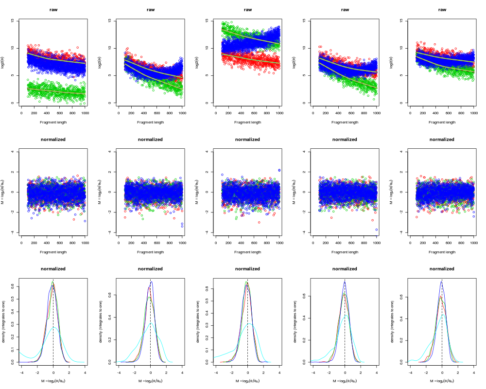
# Plot raw data
xlim <- c(0, max(fl, na.rm=TRUE));
ylim <- c(0, max(log2(theta), na.rm=TRUE));
Mlim <- c(-1,1)*4;
xlab <- "Fragment length";
ylab <- expression(log2(theta));
Mlab <- expression(M==log[2](theta/theta[R]));

layout(matrix(1:(3*I), ncol=I, byrow=TRUE));
for (ii in 1:I) {
  plot(NA, xlim=xlim, ylim=ylim, xlab=xlab, ylab=ylab, main="raw");

  # Single-enzyme units
  for (ee in 1:2) {
    # The raw data
    uu <- unitSets[[ee]];
    points(fl[uu,ee], log2(theta[uu,ii]), col=ee+1);
  }

  # Both-enzyme units (use fragment-length for enzyme #1)
  uu <- unitSets$both;
  points(fl[uu,1], log2(theta[uu,ii]), col=3+1);

  for (ee in 1:2) {
    # The true effects
    uu <- unitSets[[ee]];
    lines(lowess(fl[uu,ee], log2(theta[uu,ii])), col="black", lwd=4, lty=3);

    # The estimated effects
    fit <- fits[[ii]][[ee]]$fit;
    lines(fit, col="orange", lwd=3);

    muT <- targetFcns[[ee]](fl[uu,ee]);
    lines(fl[uu,ee], muT, col="cyan", lwd=1);
  }
}

# Calculate log-ratios
thetaR <- rowMeans(thetaN, na.rm=TRUE);
M <- log2(thetaN/thetaR);

# Plot normalized data
for (ii in 1:I) {
  plot(NA, xlim=xlim, ylim=Mlim, xlab=xlab, ylab=Mlab, main="normalized");
  # Single-enzyme units
  for (ee in 1:2) {
    # The normalized data
    uu <- unitSets[[ee]];
    points(fl[uu,ee], M[uu,ii], col=ee+1);
  }
  # Both-enzyme units (use fragment-length for enzyme #1)
  uu <- unitSets$both;
  points(fl[uu,1], M[uu,ii], col=3+1);
}

ylim <- c(0,1.5);
for (ii in 1:I) {
  data <- list();
  for (ee in 1:2) {
    # The normalized data
    uu <- unitSets[[ee]];
    data[[ee]] <- M[uu,ii];
  }
  uu <- unitSets$both;
  if (length(uu) > 0)
    data[[3]] <- M[uu,ii];

  uu <- unitSets$none;
  if (length(uu) > 0)
    data[[4]] <- M[uu,ii];

  cols <- seq(along=data)+1;
  plotDensity(data, col=cols, xlim=Mlim, xlab=Mlab, main="normalized");

  abline(v=0, lty=2);
}

Results


R version 3.3.1 (2016-06-21) -- "Bug in Your Hair"
Copyright (C) 2016 The R Foundation for Statistical Computing
Platform: x86_64-pc-linux-gnu (64-bit)

R is free software and comes with ABSOLUTELY NO WARRANTY.
You are welcome to redistribute it under certain conditions.
Type 'license()' or 'licence()' for distribution details.

R is a collaborative project with many contributors.
Type 'contributors()' for more information and
'citation()' on how to cite R or R packages in publications.

Type 'demo()' for some demos, 'help()' for on-line help, or
'help.start()' for an HTML browser interface to help.
Type 'q()' to quit R.

> library(aroma.light)
aroma.light v3.2.0 (2016-01-06) successfully loaded. See ?aroma.light for help.
> png(filename="/home/ddbj/snapshot/RGM3/R_BC/result/aroma.light/normalizeFragmentLength.Rd_%03d_medium.png", width=480, height=480)
> ### Name: normalizeFragmentLength
> ### Title: Normalizes signals for PCR fragment-length effects
> ### Aliases: normalizeFragmentLength.default normalizeFragmentLength
> ### Keywords: nonparametric robust
> 
> ### ** Examples
> 
>   # - - - - - - - - - - - - - - - - - - - - - - - - - - - - - - - - - -
> # Example 1: Single-enzyme fragment-length normalization of 6 arrays
> # - - - - - - - - - - - - - - - - - - - - - - - - - - - - - - - - - -
> # Number samples
> I <- 9;
> 
> # Number of loci
> J <- 1000;
> 
> # Fragment lengths
> fl <- seq(from=100, to=1000, length.out=J);
> 
> # Simulate data points with unknown fragment lengths
> hasUnknownFL <- seq(from=1, to=J, by=50);
> fl[hasUnknownFL] <- NA;
> 
> # Simulate data
> y <- matrix(0, nrow=J, ncol=I);
> maxY <- 12;
> for (kk in 1:I) {
+   k <- runif(n=1, min=3, max=5);
+   mu <- function(fl) {
+     mu <- rep(maxY, length(fl));
+     ok <- !is.na(fl);
+     mu[ok] <- mu[ok] - fl[ok]^{1/k};
+     mu;
+   }
+   eps <- rnorm(J, mean=0, sd=1);
+   y[,kk] <- mu(fl) + eps;
+ }
> 
> # Normalize data (to a zero baseline)
> yN <- apply(y, MARGIN=2, FUN=function(y) {
+   normalizeFragmentLength(y, fragmentLengths=fl, onMissing="median");
+ })
> 
> # The correction factors
> rho <- y-yN;
> print(summary(rho));
       V1              V2              V3              V4       
 Min.   :7.435   Min.   :6.287   Min.   :5.148   Min.   :7.081  
 1st Qu.:7.757   1st Qu.:6.605   1st Qu.:5.551   1st Qu.:7.407  
 Median :8.028   Median :7.067   Median :6.080   Median :7.763  
 Mean   :8.098   Mean   :7.179   Mean   :6.258   Mean   :7.871  
 3rd Qu.:8.435   3rd Qu.:7.706   3rd Qu.:6.918   3rd Qu.:8.294  
 Max.   :8.950   Max.   :8.489   Max.   :7.941   Max.   :9.037  
       V5              V6              V7              V8       
 Min.   :5.896   Min.   :6.503   Min.   :4.223   Min.   :6.071  
 1st Qu.:6.304   1st Qu.:6.891   1st Qu.:4.881   1st Qu.:6.519  
 Median :6.765   Median :7.334   Median :5.572   Median :6.996  
 Mean   :6.888   Mean   :7.405   Mean   :5.731   Mean   :7.094  
 3rd Qu.:7.441   3rd Qu.:7.887   3rd Qu.:6.556   3rd Qu.:7.625  
 Max.   :8.259   Max.   :8.576   Max.   :7.703   Max.   :8.492  
       V9       
 Min.   :5.935  
 1st Qu.:6.431  
 Median :6.936  
 Mean   :7.050  
 3rd Qu.:7.623  
 Max.   :8.590  
> # The correction for units with unknown fragment lengths
> # equals the median correction factor of all other units
> print(summary(rho[hasUnknownFL,]));
       V1              V2              V3             V4              V5       
 Min.   :8.028   Min.   :7.067   Min.   :6.08   Min.   :7.763   Min.   :6.765  
 1st Qu.:8.028   1st Qu.:7.067   1st Qu.:6.08   1st Qu.:7.763   1st Qu.:6.765  
 Median :8.028   Median :7.067   Median :6.08   Median :7.763   Median :6.765  
 Mean   :8.028   Mean   :7.067   Mean   :6.08   Mean   :7.763   Mean   :6.765  
 3rd Qu.:8.028   3rd Qu.:7.067   3rd Qu.:6.08   3rd Qu.:7.763   3rd Qu.:6.765  
 Max.   :8.028   Max.   :7.067   Max.   :6.08   Max.   :7.763   Max.   :6.765  
       V6              V7              V8              V9       
 Min.   :7.334   Min.   :5.572   Min.   :6.996   Min.   :6.936  
 1st Qu.:7.334   1st Qu.:5.572   1st Qu.:6.996   1st Qu.:6.936  
 Median :7.334   Median :5.572   Median :6.996   Median :6.936  
 Mean   :7.334   Mean   :5.572   Mean   :6.996   Mean   :6.936  
 3rd Qu.:7.334   3rd Qu.:5.572   3rd Qu.:6.996   3rd Qu.:6.936  
 Max.   :7.334   Max.   :5.572   Max.   :6.996   Max.   :6.936  
> 
> # Plot raw data
> layout(matrix(1:9, ncol=3));
> xlim <- c(0,max(fl, na.rm=TRUE));
> ylim <- c(0,max(y, na.rm=TRUE));
> xlab <- "Fragment length";
> ylab <- expression(log2(theta));
> for (kk in 1:I) {
+   plot(fl, y[,kk], xlim=xlim, ylim=ylim, xlab=xlab, ylab=ylab);
+   ok <- (is.finite(fl) & is.finite(y[,kk]));
+   lines(lowess(fl[ok], y[ok,kk]), col="red", lwd=2);
+ }
> 
> # Plot normalized data
> layout(matrix(1:9, ncol=3));
> ylim <- c(-1,1)*max(y, na.rm=TRUE)/2;
> for (kk in 1:I) {
+   plot(fl, yN[,kk], xlim=xlim, ylim=ylim, xlab=xlab, ylab=ylab);
+   ok <- (is.finite(fl) & is.finite(y[,kk]));
+   lines(lowess(fl[ok], yN[ok,kk]), col="blue", lwd=2);
+ }
> 
> 
>   # - - - - - - - - - - - - - - - - - - - - - - - - - - - - - - - - - -
> # Example 2: Two-enzyme fragment-length normalization of 6 arrays
> # - - - - - - - - - - - - - - - - - - - - - - - - - - - - - - - - - -
> set.seed(0xbeef);
> 
> # Number samples
> I <- 5;
> 
> # Number of loci
> J <- 3000;
> 
> # Fragment lengths (two enzymes)
> fl <- matrix(0, nrow=J, ncol=2);
> fl[,1] <- seq(from=100, to=1000, length.out=J);
> fl[,2] <- seq(from=1000, to=100, length.out=J);
> 
> # Let 1/2 of the units be on both enzymes
> fl[seq(from=1, to=J, by=4),1] <- NA;
> fl[seq(from=2, to=J, by=4),2] <- NA;
> 
> # Let some have unknown fragment lengths
> hasUnknownFL <- seq(from=1, to=J, by=15);
> fl[hasUnknownFL,] <- NA;
> 
> # Sty/Nsp mixing proportions:
> rho <- rep(1, I);
> rho[1] <- 1/3;  # Less Sty in 1st sample
> rho[3] <- 3/2;  # More Sty in 3rd sample
> 
> 
> # Simulate data
> z <- array(0, dim=c(J,2,I));
> maxLog2Theta <- 12;
> for (ii in 1:I) {
+   # Common effect for both enzymes
+   mu <- function(fl) {
+     k <- runif(n=1, min=3, max=5);
+     mu <- rep(maxLog2Theta, length(fl));
+     ok <- is.finite(fl);
+     mu[ok] <- mu[ok] - fl[ok]^{1/k};
+     mu;
+   }
+ 
+   # Calculate the effect for each data point
+   for (ee in 1:2) {
+     z[,ee,ii] <- mu(fl[,ee]);
+   }
+ 
+   # Update the Sty/Nsp mixing proportions
+   ee <- 2;
+   z[,ee,ii] <- rho[ii]*z[,ee,ii];
+ 
+   # Add random errors
+   for (ee in 1:2) {
+     eps <- rnorm(J, mean=0, sd=1/sqrt(2));
+     z[,ee,ii] <- z[,ee,ii] + eps;
+   }
+ }
> 
> 
> hasFl <- is.finite(fl);
> 
> unitSets <- list(
+   nsp  = which( hasFl[,1] & !hasFl[,2]),
+   sty  = which(!hasFl[,1] &  hasFl[,2]),
+   both = which( hasFl[,1] &  hasFl[,2]),
+   none = which(!hasFl[,1] & !hasFl[,2])
+ )
> 
> # The observed data is a mix of two enzymes
> theta <- matrix(NA, nrow=J, ncol=I);
> 
> # Single-enzyme units
> for (ee in 1:2) {
+   uu <- unitSets[[ee]];
+   theta[uu,] <- 2^z[uu,ee,];
+ }
> 
> # Both-enzyme units (sum on intensity scale)
> uu <- unitSets$both;
> theta[uu,] <- (2^z[uu,1,]+2^z[uu,2,])/2;
> 
> # Missing units (sample from the others)
> uu <- unitSets$none;
> theta[uu,] <- apply(theta, MARGIN=2, sample, size=length(uu))
> 
> # Calculate target array
> thetaT <- rowMeans(theta, na.rm=TRUE);
> targetFcns <- list();
> for (ee in 1:2) {
+   uu <- unitSets[[ee]];
+   fit <- lowess(fl[uu,ee], log2(thetaT[uu]));
+   class(fit) <- "lowess";
+   targetFcns[[ee]] <- function(fl, ...) {
+     predict(fit, newdata=fl);
+   }
+ }
> 
> 
> # Fit model only to a subset of the data
> subsetToFit <- setdiff(1:J, seq(from=1, to=J, by=10))
> 
> # Normalize data (to a target baseline)
> thetaN <- matrix(NA, nrow=J, ncol=I);
> fits <- vector("list", I);
> for (ii in 1:I) {
+   lthetaNi <- normalizeFragmentLength(log2(theta[,ii]), targetFcns=targetFcns,
+                      fragmentLengths=fl, onMissing="median",
+                      subsetToFit=subsetToFit, .returnFit=TRUE);
+   fits[[ii]] <- attr(lthetaNi, "modelFit");
+   thetaN[,ii] <- 2^lthetaNi;
+ }
> 
> 
> # Plot raw data
> xlim <- c(0, max(fl, na.rm=TRUE));
> ylim <- c(0, max(log2(theta), na.rm=TRUE));
> Mlim <- c(-1,1)*4;
> xlab <- "Fragment length";
> ylab <- expression(log2(theta));
> Mlab <- expression(M==log[2](theta/theta[R]));
> 
> layout(matrix(1:(3*I), ncol=I, byrow=TRUE));
> for (ii in 1:I) {
+   plot(NA, xlim=xlim, ylim=ylim, xlab=xlab, ylab=ylab, main="raw");
+ 
+   # Single-enzyme units
+   for (ee in 1:2) {
+     # The raw data
+     uu <- unitSets[[ee]];
+     points(fl[uu,ee], log2(theta[uu,ii]), col=ee+1);
+   }
+ 
+   # Both-enzyme units (use fragment-length for enzyme #1)
+   uu <- unitSets$both;
+   points(fl[uu,1], log2(theta[uu,ii]), col=3+1);
+ 
+   for (ee in 1:2) {
+     # The true effects
+     uu <- unitSets[[ee]];
+     lines(lowess(fl[uu,ee], log2(theta[uu,ii])), col="black", lwd=4, lty=3);
+ 
+     # The estimated effects
+     fit <- fits[[ii]][[ee]]$fit;
+     lines(fit, col="orange", lwd=3);
+ 
+     muT <- targetFcns[[ee]](fl[uu,ee]);
+     lines(fl[uu,ee], muT, col="cyan", lwd=1);
+   }
+ }
> 
> # Calculate log-ratios
> thetaR <- rowMeans(thetaN, na.rm=TRUE);
> M <- log2(thetaN/thetaR);
> 
> # Plot normalized data
> for (ii in 1:I) {
+   plot(NA, xlim=xlim, ylim=Mlim, xlab=xlab, ylab=Mlab, main="normalized");
+   # Single-enzyme units
+   for (ee in 1:2) {
+     # The normalized data
+     uu <- unitSets[[ee]];
+     points(fl[uu,ee], M[uu,ii], col=ee+1);
+   }
+   # Both-enzyme units (use fragment-length for enzyme #1)
+   uu <- unitSets$both;
+   points(fl[uu,1], M[uu,ii], col=3+1);
+ }
> 
> ylim <- c(0,1.5);
> for (ii in 1:I) {
+   data <- list();
+   for (ee in 1:2) {
+     # The normalized data
+     uu <- unitSets[[ee]];
+     data[[ee]] <- M[uu,ii];
+   }
+   uu <- unitSets$both;
+   if (length(uu) > 0)
+     data[[3]] <- M[uu,ii];
+ 
+   uu <- unitSets$none;
+   if (length(uu) > 0)
+     data[[4]] <- M[uu,ii];
+ 
+   cols <- seq(along=data)+1;
+   plotDensity(data, col=cols, xlim=Mlim, xlab=Mlab, main="normalized");
+ 
+   abline(v=0, lty=2);
+ }
> 
> 
> 
> 
> 
> 
> 
> dev.off()
null device 
          1 
>