Normalizes the empirical distribution of one of more samples to a target distribution

Description

Normalizes the empirical distribution of one of more samples to a target distribution.

The average sample distribution is calculated either robustly or not by utilizing either weightedMedian() or weighted.mean(). A weighted method is used if any of the weights are different from one.

Usage

## S3 method for class 'numeric'
normalizeQuantileRank(x, xTarget, ties=FALSE, ...)
## S3 method for class 'list'
normalizeQuantileRank(X, xTarget=NULL, ...)
## Default S3 method:
normalizeQuantile(x, ...)

Arguments

Value

Returns an object of the same shape as the input argument.

Missing values

Missing values are excluded when estimating the "common" (the baseline). Values that are NA remain NA after normalization. No new NAs are introduced.

Weights

Currently only channel weights are support due to the way quantile normalization is done. If signal weights are given, channel weights are calculated from these by taking the mean of the signal weights in each channel.

Author(s)

Adopted from Gordon Smyth (http://www.statsci.org/) in 2002 & 2006. Original code by Ben Bolstad at Statistics Department, University of California.

See Also

To calculate a target distribution from a set of samples, see averageQuantile(). For an alternative empirical density normalization methods, see normalizeQuantileSpline().

Examples

# Simulate ten samples of different lengths
N <- 10000
X <- list()
for (kk in 1:8) {
  rfcn <- list(rnorm, rgamma)[[sample(2, size=1)]]
  size <- runif(1, min=0.3, max=1)
  a <- rgamma(1, shape=20, rate=10)
  b <- rgamma(1, shape=10, rate=10)
  values <- rfcn(size*N, a, b)

  # "Censor" values
  values[values < 0 | values > 8] <- NA

  X[[kk]] <- values
}

# Add 20% missing values
X <- lapply(X, FUN=function(x) {
  x[sample(length(x), size=0.20*length(x))] <- NA;
  x
})

# Normalize quantiles
Xn <- normalizeQuantile(X)

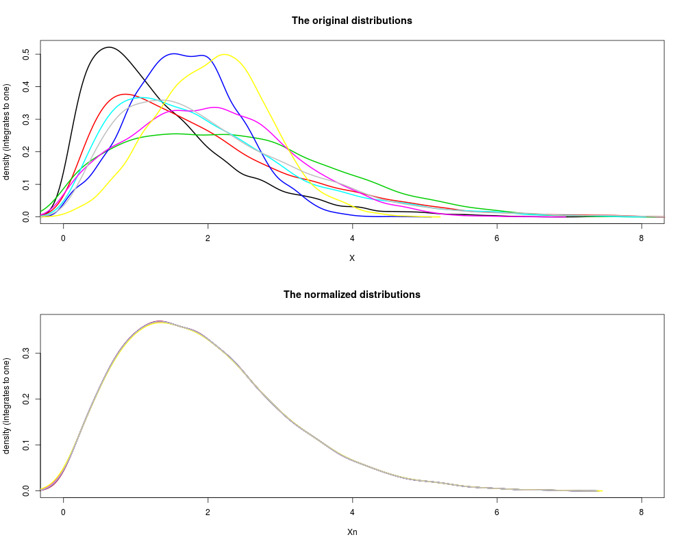
# Plot the data
layout(matrix(1:2, ncol=1))
xlim <- range(X, na.rm=TRUE);
plotDensity(X, lwd=2, xlim=xlim, main="The original distributions")
plotDensity(Xn, lwd=2, xlim=xlim, main="The normalized distributions")

Results

R version 3.3.1 (2016-06-21) -- "Bug in Your Hair"
Copyright (C) 2016 The R Foundation for Statistical Computing
Platform: x86_64-pc-linux-gnu (64-bit)

R is free software and comes with ABSOLUTELY NO WARRANTY.
You are welcome to redistribute it under certain conditions.
Type 'license()' or 'licence()' for distribution details.

R is a collaborative project with many contributors.
Type 'contributors()' for more information and
'citation()' on how to cite R or R packages in publications.

Type 'demo()' for some demos, 'help()' for on-line help, or
'help.start()' for an HTML browser interface to help.
Type 'q()' to quit R.

> library(aroma.light)
aroma.light v3.2.0 (2016-01-06) successfully loaded. See ?aroma.light for help.
> png(filename="/home/ddbj/snapshot/RGM3/R_BC/result/aroma.light/normalizeQuantileRank.Rd_%03d_medium.png", width=480, height=480)
> ### Name: normalizeQuantileRank
> ### Title: Normalizes the empirical distribution of one of more samples to
> ###   a target distribution
> ### Aliases: normalizeQuantileRank normalizeQuantileRank.numeric
> ###   normalizeQuantileRank.list normalizeQuantile
> ###   normalizeQuantile.default
> ### Keywords: methods nonparametric multivariate robust
> 
> ### ** Examples
> 
> # Simulate ten samples of different lengths
> N <- 10000
> X <- list()
> for (kk in 1:8) {
+   rfcn <- list(rnorm, rgamma)[[sample(2, size=1)]]
+   size <- runif(1, min=0.3, max=1)
+   a <- rgamma(1, shape=20, rate=10)
+   b <- rgamma(1, shape=10, rate=10)
+   values <- rfcn(size*N, a, b)
+ 
+   # "Censor" values
+   values[values < 0 | values > 8] <- NA
+ 
+   X[[kk]] <- values
+ }
> 
> # Add 20% missing values
> X <- lapply(X, FUN=function(x) {
+   x[sample(length(x), size=0.20*length(x))] <- NA;
+   x
+ })
> 
> # Normalize quantiles
> Xn <- normalizeQuantile(X)
> 
> # Plot the data
> layout(matrix(1:2, ncol=1))
> xlim <- range(X, na.rm=TRUE);
> plotDensity(X, lwd=2, xlim=xlim, main="The original distributions")
> plotDensity(Xn, lwd=2, xlim=xlim, main="The normalized distributions")
> 
> 
> 
> 
> 
> dev.off()
null device 
          1 
>