Supported by Dr. Osamu Ogasawara and  . . |
|
Last data update: 2014.03.03 |
Backbone Tree constructionDescriptionBuilds a ‘backbone tree’ from a fitted LDA model. Usagecompute.backbone.tree(lda.results, grouping = NULL, start.group.label = NULL, absolute.width = 0, width.scale.factor = 1.2, outlier.tolerance.factor = 0.1, rooting.method = NULL, only.mst = FALSE, grouping.colors = NULL, merge.sequential.backbone = FALSE) Arguments
DetailsIn order to easily visualise the structural and temporal relationship between cells, we introduced a special type of tree structure dubbed ‘backbone tree’, defined as such: Considering a set of vertices V and a distance function over all pairs of vertices: d: V <c3><83><c2><97> V -> R+, we call backbone tree a graph, T with backbone B, such that:
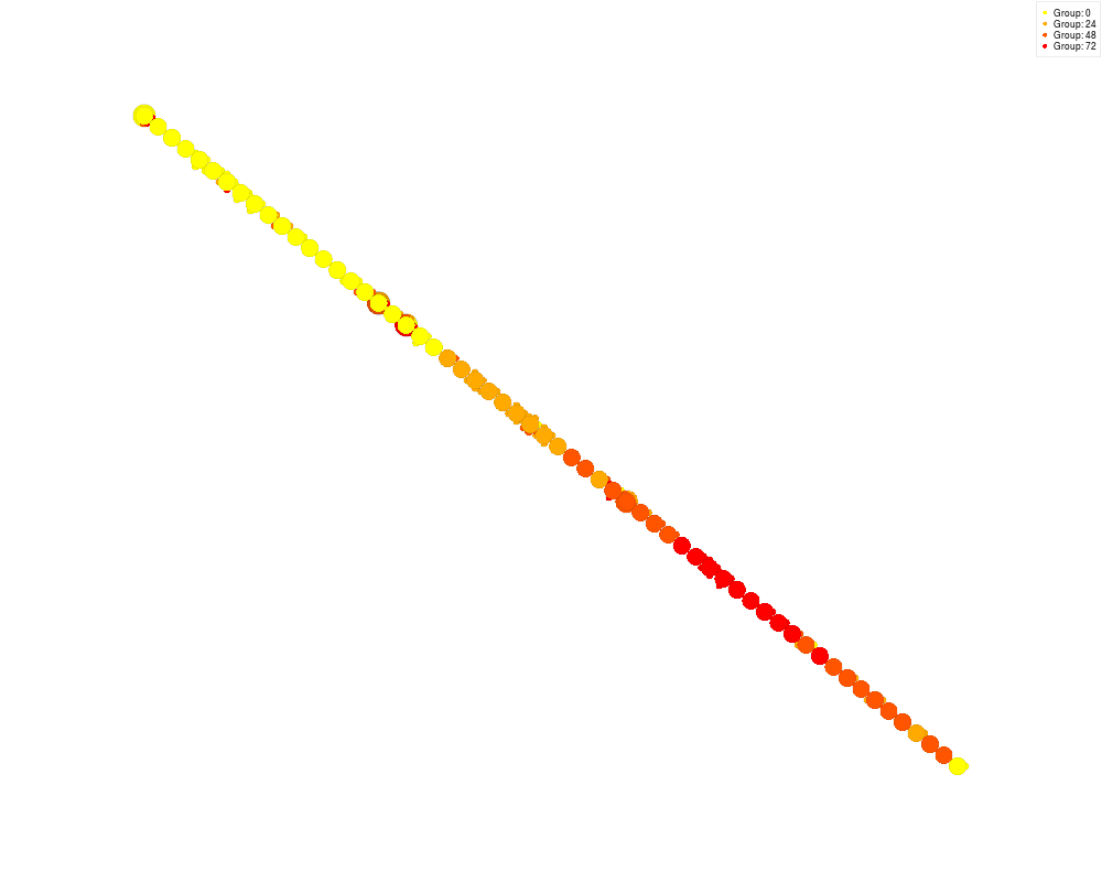
In this instance, we relax the last condition to cover only ‘most’ non-backbone vertices, allowing for a variable proportion of outliers at distance > δ from any vertices in V_B. We can then define the ‘optimal’ backbone tree to be a backbone tree such that the sum of weighted edges in the backbone subtree E_B is minimal. Finding such a tree can be easily shown to be NP-Complete (by reduction to the Vertex Cover problem), but we developed a fast heuristic relying on Minimum Spanning Tree to produce a reasonable approximation. The resulting quasi-optimal backbone tree (simply referred to as ‘the’ backbone tree thereafter) gives a clear hierarchical representation of the cell relationship: the objective function puts pressure on finding a (small) group of prominent cells (the backbone) that are good representatives of major steps in the cell evolution (in time or space), while remaining cells are similar enough to their closest representative for their difference to be ignored. Such a tree provides a very clear visualisation of overall cell differentiation paths (including potential differentiation into sub-types). ValueA igraph object with either a minimum rooted spanning-tree (if Examples# Load pre-computed LDA model for skeletal myoblast RNA-Seq data from HSMMSingleCell package: data(HSMM_lda_model) # Recover sampling time (in days) for each cell: library(HSMMSingleCell) data(HSMM_sample_sheet) days.factor = HSMM_sample_sheet$Hours days = as.numeric(levels(days.factor))[days.factor] # Compute near-optimal backbone tree: b.tree = compute.backbone.tree(HSMM_lda_model, days) # Plot resulting tree with sampling time as a vertex group colour: ct.plot.grouping(b.tree) Results
R version 3.3.1 (2016-06-21) -- "Bug in Your Hair"
Copyright (C) 2016 The R Foundation for Statistical Computing
Platform: x86_64-pc-linux-gnu (64-bit)

R is free software and comes with ABSOLUTELY NO WARRANTY.
You are welcome to redistribute it under certain conditions.
Type 'license()' or 'licence()' for distribution details.

R is a collaborative project with many contributors.
Type 'contributors()' for more information and
'citation()' on how to cite R or R packages in publications.

Type 'demo()' for some demos, 'help()' for on-line help, or
'help.start()' for an HTML browser interface to help.
Type 'q()' to quit R.

> library(cellTree)
Loading required package: topGO
Loading required package: BiocGenerics
Loading required package: parallel

Attaching package: 'BiocGenerics'

The following objects are masked from 'package:parallel':

    clusterApply, clusterApplyLB, clusterCall, clusterEvalQ,
    clusterExport, clusterMap, parApply, parCapply, parLapply,
    parLapplyLB, parRapply, parSapply, parSapplyLB

The following objects are masked from 'package:stats':

    IQR, mad, xtabs

The following objects are masked from 'package:base':

    Filter, Find, Map, Position, Reduce, anyDuplicated, append,
    as.data.frame, cbind, colnames, do.call, duplicated, eval, evalq,
    get, grep, grepl, intersect, is.unsorted, lapply, lengths, mapply,
    match, mget, order, paste, pmax, pmax.int, pmin, pmin.int, rank,
    rbind, rownames, sapply, setdiff, sort, table, tapply, union,
    unique, unsplit

Loading required package: graph
Loading required package: Biobase
Welcome to Bioconductor

    Vignettes contain introductory material; view with
    'browseVignettes()'. To cite Bioconductor, see
    'citation("Biobase")', and for packages 'citation("pkgname")'.

Loading required package: GO.db
Loading required package: AnnotationDbi
Loading required package: stats4
Loading required package: IRanges
Loading required package: S4Vectors

Attaching package: 'S4Vectors'

The following objects are masked from 'package:base':

    colMeans, colSums, expand.grid, rowMeans, rowSums


Loading required package: SparseM

Attaching package: 'SparseM'

The following object is masked from 'package:base':

    backsolve


groupGOTerms: 	GOBPTerm, GOMFTerm, GOCCTerm environments built.

Attaching package: 'topGO'

The following object is masked from 'package:IRanges':

    members

> png(filename="/home/ddbj/snapshot/RGM3/R_BC/result/cellTree/compute.backbone.tree.Rd_%03d_medium.png", width=480, height=480)
> ### Name: compute.backbone.tree
> ### Title: Backbone Tree construction
> ### Aliases: compute.backbone.tree
>
> ### ** Examples
>
> # Load pre-computed LDA model for skeletal myoblast RNA-Seq data from HSMMSingleCell package:
> data(HSMM_lda_model)
>
> # Recover sampling time (in days) for each cell:
> library(HSMMSingleCell)
> data(HSMM_sample_sheet)
> days.factor = HSMM_sample_sheet$Hours
> days = as.numeric(levels(days.factor))[days.factor]
>
> # Compute near-optimal backbone tree:
> b.tree = compute.backbone.tree(HSMM_lda_model, days)
Loading required namespace: maptpx
Using start group: 0 (1)
Using rooting method: center.start.group
Using root vertex: 4
Adding branch #1:
 [1]  65  53  45   2  55  47  57  48  44   7  19  25  69  66   9  63  18  62  51
[20]  56  16  70 136 133 143  89  78 140  94 100 177 194 141 199 201 181 161 204
[39] 225 236 255 247 246 233 229 259 258 146 235 159 185 191 216 166 149  83 168
[58] 158   8
Using branch width: 0.927 (width.scale.factor: 1.2)
Outliers: 1
Total number of branches: 1 (forks: 0)
Backbone fork merge (width: 0.927): 60 ->  60
Ranking all cells...
> # Plot resulting tree with sampling time as a vertex group colour:
> ct.plot.grouping(b.tree)
Computing tree layout...
IGRAPH DNW- 271 270 --
+ attr: grouping.colors (g/c), grouping.labels (g/n), ordered.branches
| (g/x), ratio (g/n), is.backbone (v/l), is.root (v/l), name (v/n),
| color (v/c), group.idx (v/n), grouping.label (v/n), pie (v/x), shape
| (v/c), cell.name (v/c), x (v/n), y (v/n), size (v/n), weight (e/n),
| arrow.mode (e/n)
+ edges (vertex names):
 [1]  2-> 20  2-> 26  2-> 50  2-> 55  4->  1  4-> 10  4-> 13  4-> 15  4-> 24
[10]  4-> 28  4-> 30  4-> 31  4-> 34  4-> 40  4-> 41  4-> 49  4-> 58  4-> 59
[19]  4-> 60  4-> 64  4-> 65  4->150  4->196  4->234  4->242  4->266  4->267
[28]  7-> 19  7-> 73  7->211  8-> 42  9-> 27  9-> 63  9-> 68 16-> 70 18-> 22
+ ... omitted several edges
>
>
>
>
>
> dev.off()
null device
          1
>
|