An igraph tree, as returned by compute.backbone.tree
file.output
String (optional). Path of a file where the plot should be saved in PDF format (rendered to screen if omitted).
show.labels
Boolean (optional). Whether to write each cell's row number next to its vertex.
force.recompute.layout
Boolean (optional). If set to TRUE, recomputes the graph's layout coordinates even when present.
height, width
Numeric (optional). Height and width (in inches) of the plot.
vertebrae.distance
Numeric (optional). If non-zero: forces a specific plotting distance (in pixels) between backbone cells and related peripheral cells (‘vertebrae’).
backbone.vertex.size, vert.vertex.size
Numeric (optional). Diameter (in pixels) of backbone and vertebrae cell vertices.
Value
An updated igraph object with x and y vertex coordinate attributes.
Examples
# Load pre-computed LDA model for skeletal myoblast RNA-Seq data from HSMMSingleCell package:
data(HSMM_lda_model)
# Recover sampling time (in days) for each cell:
library(HSMMSingleCell)
data(HSMM_sample_sheet)
days.factor = HSMM_sample_sheet$Hours
days = as.numeric(levels(days.factor))[days.factor]
# Compute near-optimal backbone tree:
b.tree = compute.backbone.tree(HSMM_lda_model, days)
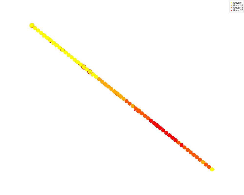
# Plot resulting tree with sampling time as a vertex group colour:
ct.plot.grouping(b.tree)
Results
R version 3.3.1 (2016-06-21) -- "Bug in Your Hair"
Copyright (C) 2016 The R Foundation for Statistical Computing
Platform: x86_64-pc-linux-gnu (64-bit)

R is free software and comes with ABSOLUTELY NO WARRANTY.
You are welcome to redistribute it under certain conditions.
Type 'license()' or 'licence()' for distribution details.

R is a collaborative project with many contributors.
Type 'contributors()' for more information and
'citation()' on how to cite R or R packages in publications.

Type 'demo()' for some demos, 'help()' for on-line help, or
'help.start()' for an HTML browser interface to help.
Type 'q()' to quit R.

> library(cellTree)
Loading required package: topGO
Loading required package: BiocGenerics
Loading required package: parallel

Attaching package: 'BiocGenerics'

The following objects are masked from 'package:parallel':

    clusterApply, clusterApplyLB, clusterCall, clusterEvalQ,
    clusterExport, clusterMap, parApply, parCapply, parLapply,
    parLapplyLB, parRapply, parSapply, parSapplyLB

The following objects are masked from 'package:stats':

    IQR, mad, xtabs

The following objects are masked from 'package:base':

    Filter, Find, Map, Position, Reduce, anyDuplicated, append,
    as.data.frame, cbind, colnames, do.call, duplicated, eval, evalq,
    get, grep, grepl, intersect, is.unsorted, lapply, lengths, mapply,
    match, mget, order, paste, pmax, pmax.int, pmin, pmin.int, rank,
    rbind, rownames, sapply, setdiff, sort, table, tapply, union,
    unique, unsplit

Loading required package: graph
Loading required package: Biobase
Welcome to Bioconductor

    Vignettes contain introductory material; view with
    'browseVignettes()'. To cite Bioconductor, see
    'citation("Biobase")', and for packages 'citation("pkgname")'.

Loading required package: GO.db
Loading required package: AnnotationDbi
Loading required package: stats4
Loading required package: IRanges
Loading required package: S4Vectors

Attaching package: 'S4Vectors'

The following objects are masked from 'package:base':

    colMeans, colSums, expand.grid, rowMeans, rowSums


Loading required package: SparseM

Attaching package: 'SparseM'

The following object is masked from 'package:base':

    backsolve


groupGOTerms: 	GOBPTerm, GOMFTerm, GOCCTerm environments built.

Attaching package: 'topGO'

The following object is masked from 'package:IRanges':

    members

> png(filename="/home/ddbj/snapshot/RGM3/R_BC/result/cellTree/ct.plot.topics.Rd_%03d_medium.png", width=480, height=480)
> ### Name: ct.plot.topics
> ### Title: Plot cell tree with topic distributions
> ### Aliases: ct.plot.topics
>
> ### ** Examples
>
> # Load pre-computed LDA model for skeletal myoblast RNA-Seq data from HSMMSingleCell package:
> data(HSMM_lda_model)
>
> # Recover sampling time (in days) for each cell:
> library(HSMMSingleCell)
> data(HSMM_sample_sheet)
> days.factor = HSMM_sample_sheet$Hours
> days = as.numeric(levels(days.factor))[days.factor]
>
> # Compute near-optimal backbone tree:
> b.tree = compute.backbone.tree(HSMM_lda_model, days)
Loading required namespace: maptpx
Using start group: 0 (1)
Using rooting method: center.start.group
Using root vertex: 4
Adding branch #1:
 [1]  65  53  45   2  55  47  57  48  44   7  19  25  69  66   9  63  18  62  51
[20]  56  16  70 136 133 143  89  78 140  94 100 177 194 141 199 201 181 161 204
[39] 225 236 255 247 246 233 229 259 258 146 235 159 185 191 216 166 149  83 168
[58] 158   8
Using branch width: 0.927 (width.scale.factor: 1.2)
Outliers: 1
Total number of branches: 1 (forks: 0)
Backbone fork merge (width: 0.927): 60 ->  60
Ranking all cells...
> # Plot resulting tree with sampling time as a vertex group colour:
> ct.plot.grouping(b.tree)
Computing tree layout...
IGRAPH DNW- 271 270 --
+ attr: grouping.colors (g/c), grouping.labels (g/n), ordered.branches
| (g/x), ratio (g/n), is.backbone (v/l), is.root (v/l), name (v/n),
| color (v/c), group.idx (v/n), grouping.label (v/n), pie (v/x), shape
| (v/c), cell.name (v/c), x (v/n), y (v/n), size (v/n), weight (e/n),
| arrow.mode (e/n)
+ edges (vertex names):
 [1]  2-> 20  2-> 26  2-> 50  2-> 55  4->  1  4-> 10  4-> 13  4-> 15  4-> 24
[10]  4-> 28  4-> 30  4-> 31  4-> 34  4-> 40  4-> 41  4-> 49  4-> 58  4-> 59
[19]  4-> 60  4-> 64  4-> 65  4->150  4->196  4->234  4->242  4->266  4->267
[28]  7-> 19  7-> 73  7->211  8-> 42  9-> 27  9-> 63  9-> 68 16-> 70 18-> 22
+ ... omitted several edges
>
>
>
>
>
> dev.off()
null device
          1
>
 .
.