R Graphical Manual

Browse All

Last data update: 2014.03.03

R: Construction of the superclusters and the one-to-one mapping...

SCmapping

R Documentation

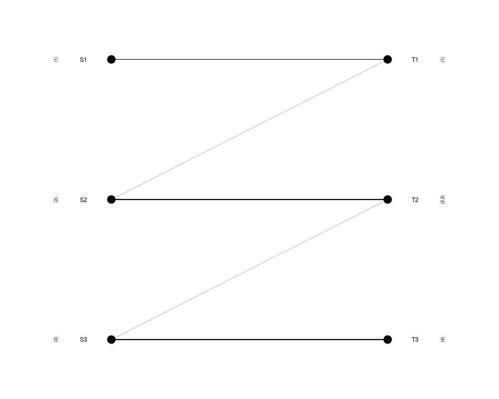
Construction of the superclusters and the one-to-one mapping between them

Description

SPmapping identifies groups of clusters from two flat partitionings that have the largest common intersections. These groups are found by following a greedy strategy: all edges incident to each cluster are removed except for the one(s) with highest weight; then the connected components in the resulting bi-graph define the correspondences of superclusters.

Usage

SCmapping(clustering1, clustering2, plotting = TRUE, h.min = 0.1, line.wd = 3, 
    point.sz = 3, offset = 0.1, evenly = TRUE, horiz = FALSE, max.iter =24, 
    node.col = NULL, edge.col = NULL,...)

Arguments

`clustering1`	a vector indicating the cluster in which each point is allocated in the first flat partitioning.
`clustering2`	a vector indicating the cluster in which each point is allocated in the second flat partitioning.
`plotting`	a Boolean parameter which leads to the representation of the bi-graph if TRUE.
`h.min`	the minimum separation between nodes in the same layer; if the barycentre algorithm sets two nodes to be less than this distance apart, then the second node and the following ones are shifted (downwards, in the vertical layout, and to the right, in the horizontal layout).
`line.wd`	a numerical parameter that fixes the width of the thickest edge, according to the weights; 3 by default.
`point.sz`	a numerical parameter that fixes the size of the nodes in the bi-graph; 2 by default.
`offset`	a numerical parameter that sets the separation between the nodes and their labels. It is set to 0.1 by default.
`evenly`	a Boolean parameter; if TRUE the coordinate values are ignored, and the nodes are drawn evenly spaced, according to the ordering obtained by the barycentre algorithm. It is set to FALSE by default.
`horiz`	a Boolean argument for vertical (default) or horizontal layout.
`max.iter`	an integer stating the maximum number of runs of the barycentre heuristic on both layers of the bi-graph.
`node.col`	defines the colour of nodes from both layers.
`edge.col`	sets the colour of the edges.
`...`	further graphical parameters can be passed to the function.

Details

The one-to-one mapping between groups of clusters from two different flat partitionings is computed with a greedy algorithm: firstly, for each node the edge with the highest weight is taken, and secondly, the connected components in the edge-reduced bi-graph are found, so that each connected component corresponds to a pair of superclusters with a large overlap.

Value

a list containing:

`s.clustering1`	a vector indicating the supercluster in which each point is allocated in the first superclustering.
`s.clustering2`	a vector indicating the supercluster in which each point is allocated in the second superclustering.
`merging1`	a list of p elements, whose j-th component contains the labels of the initial clusters from the first partitioning that have been merged to produce the j-th supercluster in the left layer of the bi- graph.
`merging2`	a list of p elements, whose j-th component contains the labels of the initial clusters from the second partitioning that have been merged to produce the j-th supercluster in the right layer of the bi- graph.
`weights`	a `pxp` matrix containing the size of the intersections between the superclusters.

Author(s)

Aurora Torrente aurora@ebi.ac.uk and Alvis Brazma brazma@ebi.ac.uk

References

Torrente, A. et al. (2005). A new algorithm for comparing and visualizing relationships between hierarchical and flat gene expression data clusterings. Bioinformatics, 21 (21), 3993-3999.

Examples

### computation and visualisation of superclusters
    # simulated data
    clustering1 <- c(rep(1, 5), rep(2, 10), rep(3, 10))
    clustering2 <- c(rep(1, 6), rep(2, 6), rep(3, 4), rep(4, 9))
    mapping <- SCmapping(clustering1, clustering2)

Results


R version 3.3.1 (2016-06-21) -- "Bug in Your Hair"
Copyright (C) 2016 The R Foundation for Statistical Computing
Platform: x86_64-pc-linux-gnu (64-bit)

R is free software and comes with ABSOLUTELY NO WARRANTY.
You are welcome to redistribute it under certain conditions.
Type 'license()' or 'licence()' for distribution details.

R is a collaborative project with many contributors.
Type 'contributors()' for more information and
'citation()' on how to cite R or R packages in publications.

Type 'demo()' for some demos, 'help()' for on-line help, or
'help.start()' for an HTML browser interface to help.
Type 'q()' to quit R.

> library(clustComp)
> png(filename="/home/ddbj/snapshot/RGM3/R_BC/result/clustComp/SCmapping.Rd_%03d_medium.png", width=480, height=480)
> ### Name: SCmapping
> ### Title: Construction of the superclusters and the one-to-one mapping
> ###   between them
> ### Aliases: SCmapping
> ### Keywords: clustering comparison
> 
> ### ** Examples
> 
> ### computation and visualisation of superclusters
>     # simulated data
>     clustering1 <- c(rep(1, 5), rep(2, 10), rep(3, 10))
>     clustering2 <- c(rep(1, 6), rep(2, 6), rep(3, 4), rep(4, 9))
>     mapping <- SCmapping(clustering1, clustering2)
> 
> 
> 
> 
> 
> dev.off()
null device 
          1 
>