R Graphical Manual

Browse All

Last data update: 2014.03.03

R: Plot the bi-graph determined by the branches in the tree and...

drawTreeGraph

R Documentation

Plot the bi-graph determined by the branches in the tree and the flat clusters

Description

drawTreeGraph plots both a hierarchical tree, either complete or pruned, and a flat clustering, connected with edges whose thickness is proportional to the number of elements shared by branches and clusters, to form a weighted bi-graph. Its usage is mainly internal, as part of the visualisation of the hierarchical.look.ahead function. The size of each cluster is also displayed.

Usage

drawTreeGraph(weight, current.order, coordinates, tree, dot = TRUE, 
    line.wd = 3, main = NULL, expanded = FALSE, hclust.obj = NULL, 
    labels = NULL, cex.labels = 1)

Arguments

`weight`	a contingency matrix containing the intersection sizes (edge weights) between branches in the tree and clusters from the flat partitioning.
`current.order`	a list of two components; the first one is a vector with the branches (rows of the matrix `weight`) in the ordering in which they are drawn; the second one provides the ordering for flat clusters (columns of `weight`). Both are drawn from bottom upwards.
`coordinates`	a list of two components; the first one is a vector providing the Y-coordinates, from bottom upwards, for the branches, whereas the second one provides the Y-coordinates, from bottom upwards, for the flat clusters.
`tree`	a list with two components: `$heights`, a vector describing the heights at which the different branches in the tree are agglomerated, and `$branches`, a matrix of 3 columns; the i-th row contains as first element the branch split at the i-th allowed splitting, and as second and third elements, the corresponding children.
`dot`	a Boolean parameter; if TRUE then the last split in the children-tree is shown with a red open circle.
`line.wd`	a number indicating the width of the thickest edge(s) in the bigraph.
`main`	a character string for the plot title.
`expanded`	a Boolean parameter indicating whether the hierarchical tree should be plotted complete or with its branches collapsed.
`hclust.obj`	an hclust object describing the how the leaves are merged and the ordering of the branches, which might have been changed by the gravity-centre algorithm.
`labels`	a vector indicating the labels for the leaves in the expanded tree.
`cex.labels`	a number indicating the magnification used for the labels of the leaves.

Details

The drawTreeGraph allows visualising the comparison of a hierarchical clustering, drawn on the left hand side of the plot, and a flat clustering, represented on the right hand side. The tree branches are labelled by their original labels preceded by 'B'; if the function is called as part of the flatVShier algorithm, then the standard notation for initial branch labels is that of hclust objects: if the label is a negative integer it corresponds to a leaf; if it is a positive integer, then it corresponds to a branch that agglomerates at least two elements, and the number represent the stage at which the branch was formed. The last splitting can be optionally highlighted with a red open circle upon the parent-node. The flat clusters are labelled by their original labels preceded by 'F'.

Value

a list of components including:

`b.coord`	a vector indicating the Y coordinates of the nodes in the bi-graph representing the branches of the hierarchical tree.
`f.coord`	a vector indicating the Y coordinates of the nodes in the bi-graph representing the flat clusters.
`x.coords`	a vector of two components indicating the X coordinates at which each layer of the bi-graph is represented.

Author(s)

Aurora Torrente aurora@ebi.ac.uk and Alvis Brazma brazma@ebi.ac.uk

References

Torrente, A. et al. (2005). A new algorithm for comparing and visualizing relationships between hierarchical and flat gene expression data clusterings. Bioinformatics, 21 (21), 3993-3999.

Examples

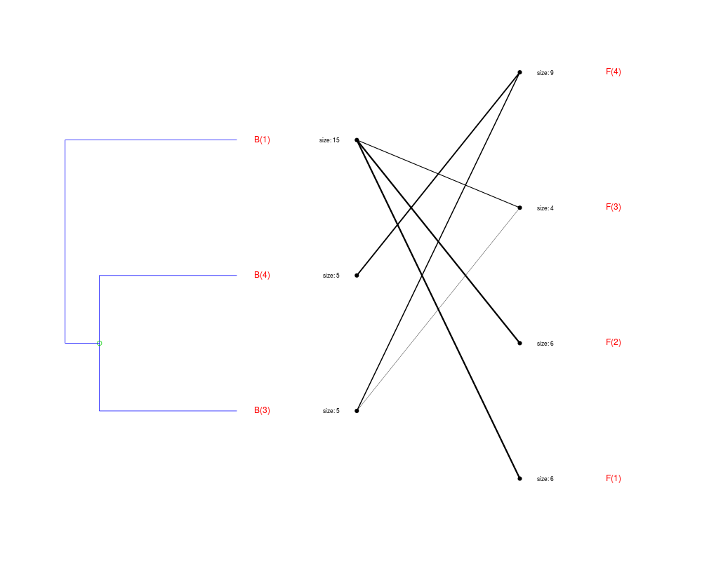
    ### simulated data
    parent.clustering <- c(rep(1, 15), rep(2, 10))
    # replace the branch '2' by its children '3' and '4' 
    children.clustering <- c(rep(1, 15), rep(3, 5), rep(4, 5))
    flat.clustering <- c(rep(1, 6), rep(2, 6), rep(3, 4), rep(4, 9))
    split <- rbind(c(0, 1, 2), c(2, 3, 4))
    weight <- table(children.clustering, flat.clustering)
    current.order <- list(c(3, 4, 1), 1:4)
    coordinates <- list(c(-1, 0, 1), c(-1.5, -0.5, 0.5, 1.5))
    tree<-list(heights = c(1, 0.8), branches = split)
    drawTreeGraph(weight, current.order, coordinates, tree)

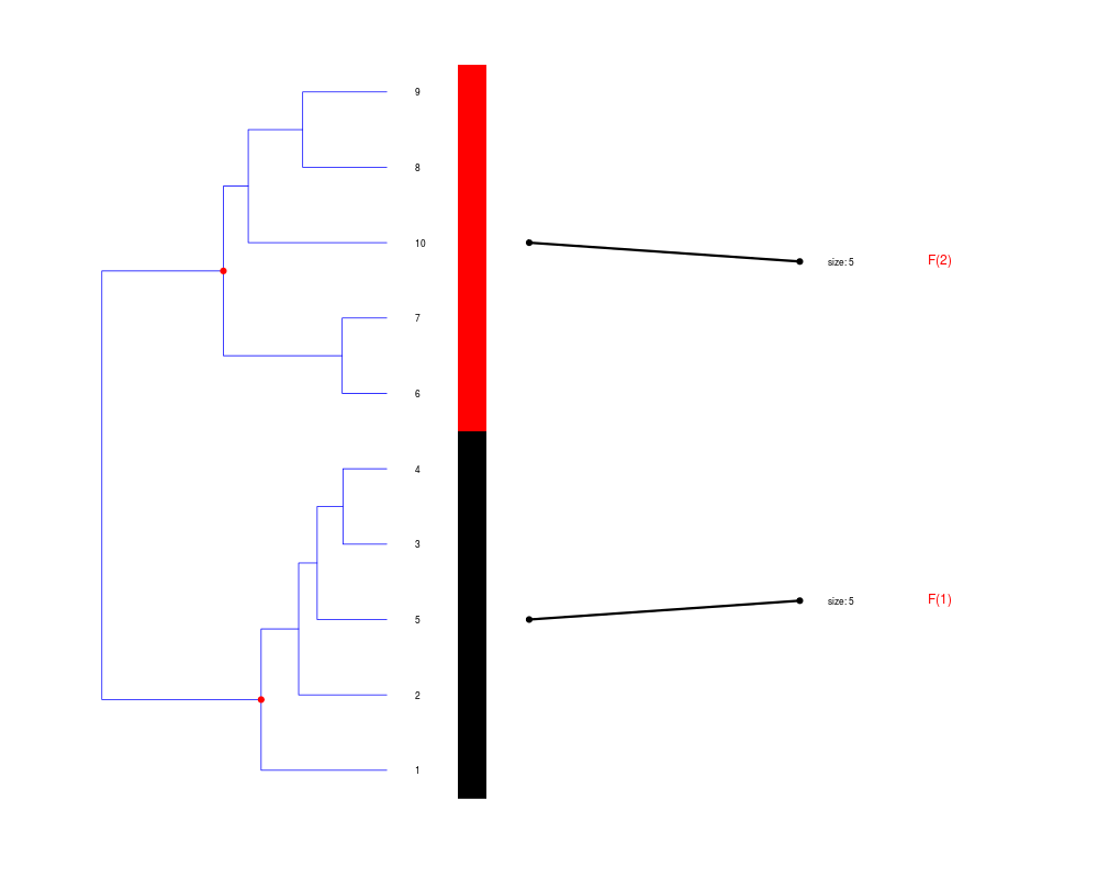
    ### expanded tree
    set.seed(0)
    myData <- matrix(rnorm(50), 10, 5)
    myData[1:5,] <- myData[1:5, ] + 2  # two groups
    flat.clustering <- kmeans(myData, 2)$cluster
    hierar.clustering <- hclust(dist(myData))
    weight <- matrix(c(5, 0, 0, 5), 2, 2)
    colnames(weight) <- 1:2; rownames(weight) <- c(6,8)
    current.order <- list(c(6, 8), 1:2)
    coordinates <- list(c(0.25, 0.75), c(0.25, 0.75))
    tree <- list(heights = hierar.clustering$height[9], 
        branches = matrix(c(9, 6, 8), 1, 3))
    drawTreeGraph(weight, current.order, coordinates, tree, 
        expanded = TRUE, hclust.obj = hierar.clustering, 
        dot = FALSE)

Results


R version 3.3.1 (2016-06-21) -- "Bug in Your Hair"
Copyright (C) 2016 The R Foundation for Statistical Computing
Platform: x86_64-pc-linux-gnu (64-bit)

R is free software and comes with ABSOLUTELY NO WARRANTY.
You are welcome to redistribute it under certain conditions.
Type 'license()' or 'licence()' for distribution details.

R is a collaborative project with many contributors.
Type 'contributors()' for more information and
'citation()' on how to cite R or R packages in publications.

Type 'demo()' for some demos, 'help()' for on-line help, or
'help.start()' for an HTML browser interface to help.
Type 'q()' to quit R.

> library(clustComp)
> png(filename="/home/ddbj/snapshot/RGM3/R_BC/result/clustComp/drawTreeGraph.Rd_%03d_medium.png", width=480, height=480)
> ### Name: drawTreeGraph
> ### Title: Plot the bi-graph determined by the branches in the tree and the
> ###   flat clusters
> ### Aliases: drawTreeGraph
> ### Keywords: clustering comparison
> 
> ### ** Examples
> 
>     ### simulated data
>     parent.clustering <- c(rep(1, 15), rep(2, 10))
>     # replace the branch '2' by its children '3' and '4' 
>     children.clustering <- c(rep(1, 15), rep(3, 5), rep(4, 5))
>     flat.clustering <- c(rep(1, 6), rep(2, 6), rep(3, 4), rep(4, 9))
>     split <- rbind(c(0, 1, 2), c(2, 3, 4))
>     weight <- table(children.clustering, flat.clustering)
>     current.order <- list(c(3, 4, 1), 1:4)
>     coordinates <- list(c(-1, 0, 1), c(-1.5, -0.5, 0.5, 1.5))
>     tree<-list(heights = c(1, 0.8), branches = split)
>     drawTreeGraph(weight, current.order, coordinates, tree)
$b.coord
[1] -1  0  1

$f.coord
   1    2    3    4 
-1.5 -0.5  0.5  1.5 

$x.coords
[1] 0.70 1.65

> 
>     ### expanded tree
>     set.seed(0)
>     myData <- matrix(rnorm(50), 10, 5)
>     myData[1:5,] <- myData[1:5, ] + 2  # two groups
>     flat.clustering <- kmeans(myData, 2)$cluster
>     hierar.clustering <- hclust(dist(myData))
>     weight <- matrix(c(5, 0, 0, 5), 2, 2)
>     colnames(weight) <- 1:2; rownames(weight) <- c(6,8)
>     current.order <- list(c(6, 8), 1:2)
>     coordinates <- list(c(0.25, 0.75), c(0.25, 0.75))
>     tree <- list(heights = hierar.clustering$height[9], 
+         branches = matrix(c(9, 6, 8), 1, 3))
>     drawTreeGraph(weight, current.order, coordinates, tree, 
+         expanded = TRUE, hclust.obj = hierar.clustering, 
+         dot = FALSE)
$b.coord
[1] 0.2222222 0.7777778

$f.coord
[1] 0.25 0.75

$x.coords
[1] 0.50 1.45

> 
> 
> 
> 
> 
> dev.off()
null device 
          1 
>