R Graphical Manual

Browse All

Last data update: 2014.03.03

R: Comparison of two flat clusterings

flatVSflat

R Documentation

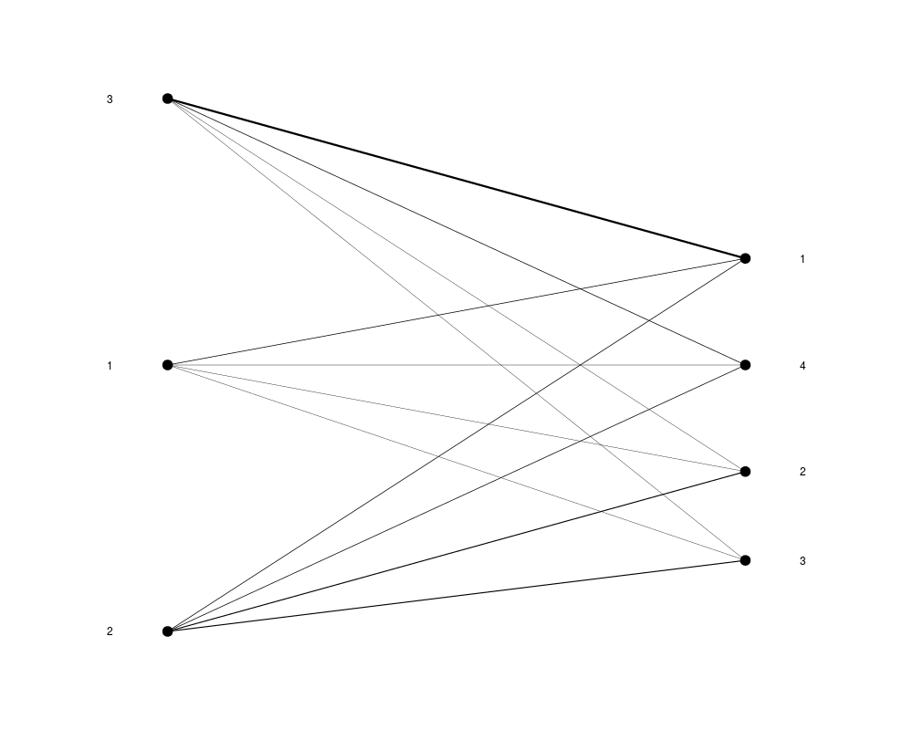
Comparison of two flat clusterings

Description

flatVSflat carries out the comparison and visualisation of two flat clusterings. The nodes in each partitioning are represented as nodes in the two layers of a bi-graph. The sizes of the intersection between clusters are reflected in the edge thickness. The number of edge crossings is minimised heuristically using the barycentre algorithm alternatively on each side.

Usage

flatVSflat(weights, coord1 = NULL, coord2 = NULL, max.iter = 24, h.min = 0.1, 
    plotting = TRUE, horiz = FALSE, offset = 0.1, line.wd = 3, point.sz = 2, 
    evenly = FALSE, main = "", xlab = "", ylab = "", col = NULL, ...)

Arguments

`weights`	a matrix containing the weights of the edges in the bigraph, which represent the overlaps between clusters in the two partitions.
`coord1`	a vector indicating the coordinates of the nodes in the first layer of the bi-graph. If not provided, then the nodes are initially equally spaced.
`coord2`	a vector indicating the coordinates of the nodes in the second layer of the bi-graph. If not provided, then the nodes are initially equally spaced.
`max.iter`	an integer stating the maximum number of runs of the barycentre heuristic on both layers of the bi-graph.
`h.min`	minimum separation between nodes in the same layer; if the barycentre algorithm sets two nodes to be less than this distance apart, then the second node and the following ones are shifted (downwards, in the vertical layout, and to the right, in the horizontal layout).
`plotting`	a Boolean parameter which yields the bi-graph if TRUE.
`horiz`	a Boolean argument for displaying a vertical (default) or horizontal layout.
`offset`	a numerical parameter that sets the separation between the nodes and their labels. It is set to 0.1 by default.
`line.wd`	a numerical parameter that fixes the width of the thickest edge(s); the rest are drawn proportionally to their weights; 3 by default.
`point.sz`	a numerical parameter that fixes the size of the nodes in the bigraph; 2 by default.
`evenly`	a Boolean parameter; if TRUE the coordinate values are ignored, and the nodes are drawn evenly spaced, according to the ordering obtained by the algorithm. It is set to FALSE by default.
`main`	graphical parameter as in `plot`.
`xlab`	graphical parameter as in `plot`.
`ylab`	graphical parameters as in `plot`.
`col`	graphical parameters as in `plot`.
`...`	further graphical parameters.

Details

As the iterations of the algorithm run the coordinates of the nodes in a single layer are updated. For a given partition, each node is assigned a new position, the gravity-centre, using the barycentre algorithm; then, the nodes in the corresponding layer are reordered according to the new positions. If the gravity-centres cause two consecutive nodes to be less than h.min apart, the coordinates of the second and all the following ones are shifted. Additionally, to improve the results of the algorithm the following strategy is also used after running the barycentre algorithm on each side: consecutive nodes are swapped if this transposition leads to a reduction in the number of edge crossings. The algorithm runs until there is no improvement in the number of crossings or until the maximum number of iterations is reached. The rownames and colnames of matrix weights contain the cluster labels. The ordering in the layout is over-imposed by the coordinate values, therefore, the names (in the coordinates) and row-/col-names (in the contingency table) should coincide.

Value

a list of components including:

`icross`	the number of edge crossings before running the barycentre algorithm.
`fcross`	the number of edge crossings after running the barycentre algorithm.
`coord1`	a vector containing the coordinates for each node in the first layer.
`coord2`	a vector containing the coordinates for each node in the second layer.

Author(s)

Aurora Torrente aurora@ebi.ac.uk and Alvis Brazma brazma@ebi.ac.uk

References

Eades, P. et al. (1986). On an edge crossing problem. Proc. of 9th Australian Computer Science Conference, pp. 327-334.

Gansner, E.R. et al. (1993). A technique for drawing directed graphs. IEEE Trans. on Software Engineering, 19 (3), 214-230.

Garey, M.R. et al. (1983). Crossing number in NP complete. SIAM J. Algebraic Discrete Methods, 4, 312-316.

Torrente, A. et al. (2005). A new algorithm for comparing and visualizing relationships between hierarchical and flat gene expression data clusterings. Bioinformatics, 21 (21), 3993-3999.

Examples

    # simulated data
    clustering1 <- c(rep(1, 5), rep(2, 10), rep(3, 10))
    clustering2 <- c(rep(1:4, 5), rep(1, 5))
    weights <- table(clustering1, clustering2)
    flatVSflat(table(clustering1, clustering2))

Results


R version 3.3.1 (2016-06-21) -- "Bug in Your Hair"
Copyright (C) 2016 The R Foundation for Statistical Computing
Platform: x86_64-pc-linux-gnu (64-bit)

R is free software and comes with ABSOLUTELY NO WARRANTY.
You are welcome to redistribute it under certain conditions.
Type 'license()' or 'licence()' for distribution details.

R is a collaborative project with many contributors.
Type 'contributors()' for more information and
'citation()' on how to cite R or R packages in publications.

Type 'demo()' for some demos, 'help()' for on-line help, or
'help.start()' for an HTML browser interface to help.
Type 'q()' to quit R.

> library(clustComp)
> png(filename="/home/ddbj/snapshot/RGM3/R_BC/result/clustComp/flatVSflat.Rd_%03d_medium.png", width=480, height=480)
> ### Name: flatVSflat
> ### Title: Comparison of two flat clusterings
> ### Aliases: flatVSflat
> ### Keywords: clustering comparison
> 
> ### ** Examples
> 
>     # simulated data
>     clustering1 <- c(rep(1, 5), rep(2, 10), rep(3, 10))
>     clustering2 <- c(rep(1:4, 5), rep(1, 5))
>     weights <- table(clustering1, clustering2)
>     flatVSflat(table(clustering1, clustering2))
$icross
[1] 91

$fcross
[1] 39

$coord1
  1   2   3 
0.8 0.5 1.1 

$coord2
   1    2    3    4 
0.92 0.68 0.58 0.80 

> 
> 
> 
> 
> 
> dev.off()
null device 
          1 
>