Supported by Dr. Osamu Ogasawara and  . . |
|
Last data update: 2014.03.03 |
Plot copy number data and/or segmentation results by sampleDescriptionPlot copy number data and/or segmentation results for each sample separately with chromosomes in different panels. Usage
plotSample(data = NULL, segments = NULL, pos.unit = "bp", sample = NULL,
            chrom = NULL, assembly = "hg19", winsoutliers = NULL, xaxis =
            "pos", layout = c(1,1), plot.ideo = TRUE, ...)
Arguments
DetailsSeveral plots may be produced on the same page with the NoteThese functions apply Author(s)Gro Nilsen See Also
Examples
#Lymphoma data
data(lymphoma)
#Take out a smaller subset of 6 samples (using subsetData):
sub.lymphoma <- subsetData(lymphoma,sample=1:6)
#Winsorize data:
wins.data <- winsorize(data=sub.lymphoma)
#Use pcf to find segments:
uni.segments <- pcf(data=wins.data,gamma=12)
#Use multipcf to find segments as well:
multi.segments <- multipcf(data=wins.data,gamma=12)
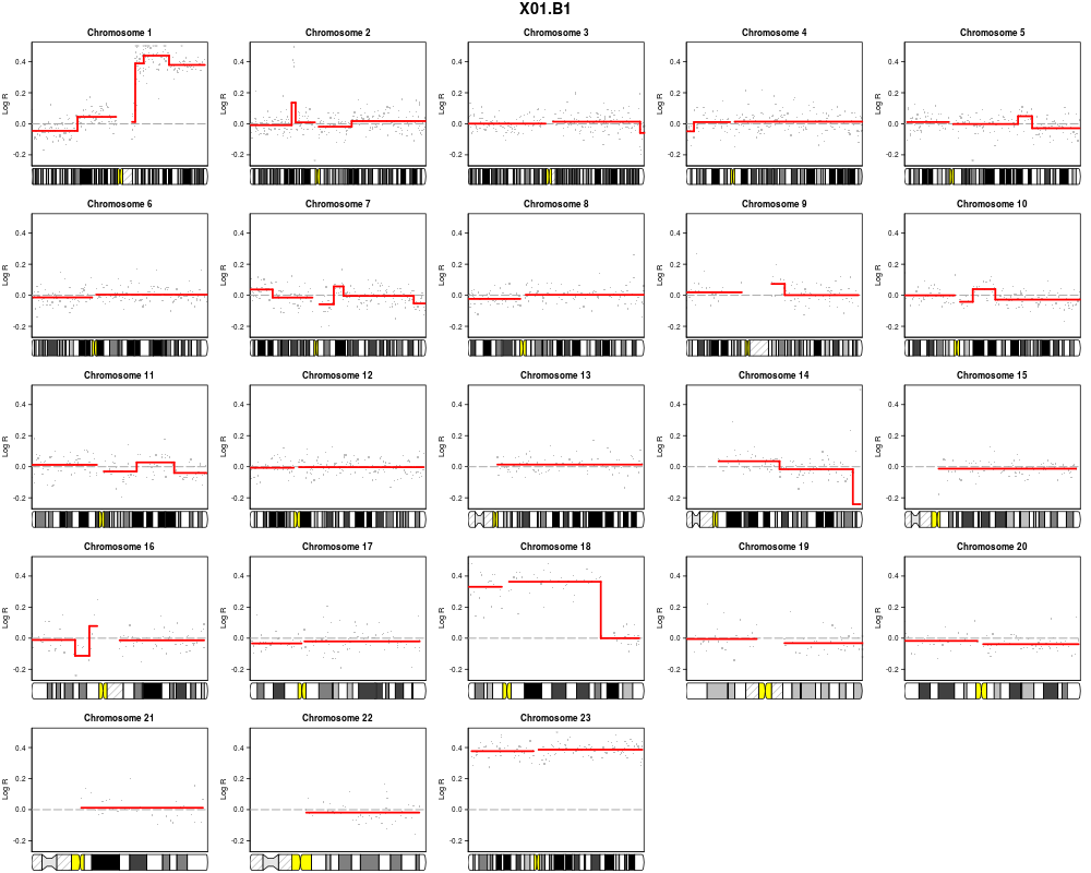
#Plot data and pcf-segments for one sample separately for each chromosome:
plotSample(data=sub.lymphoma,segments=uni.segments,sample=1,layout=c(5,5))
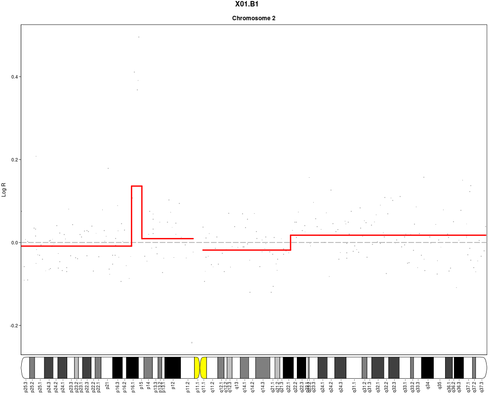
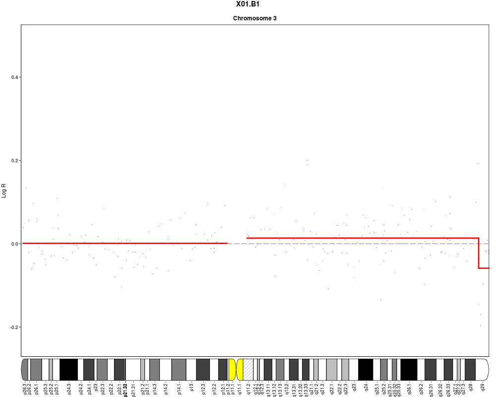
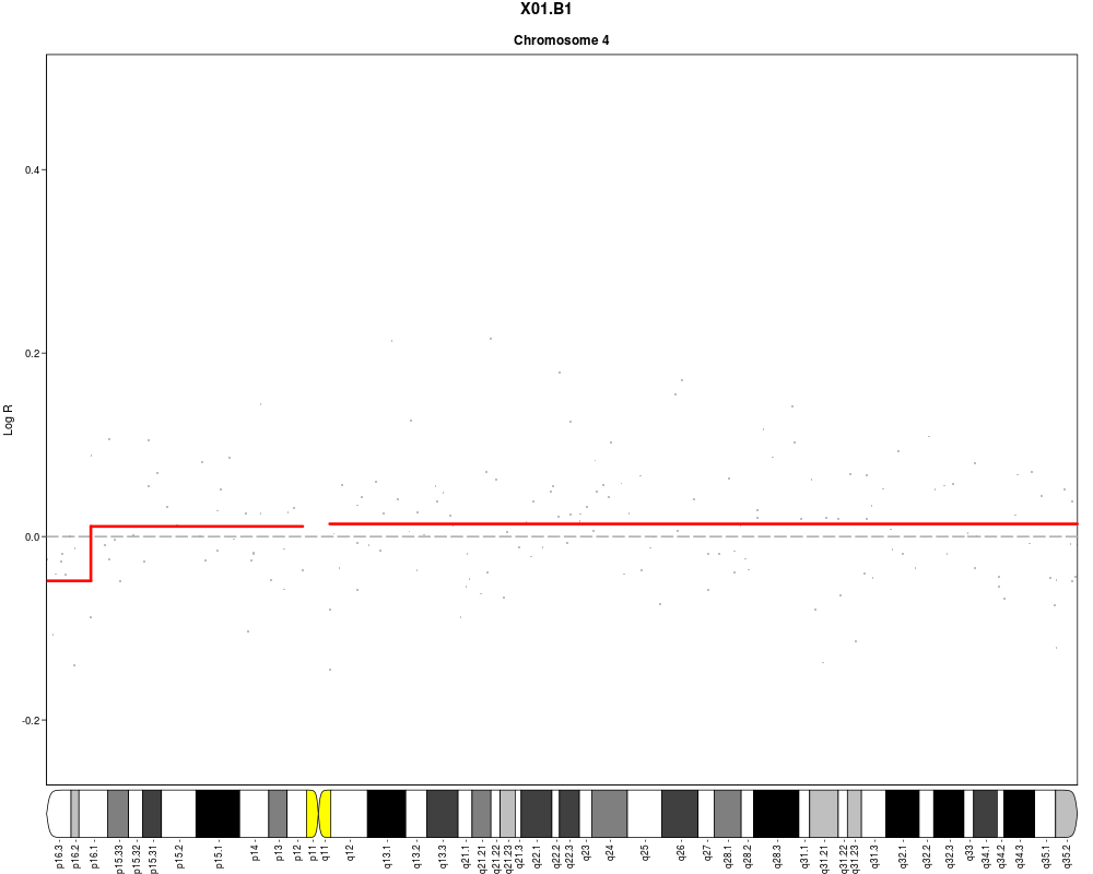
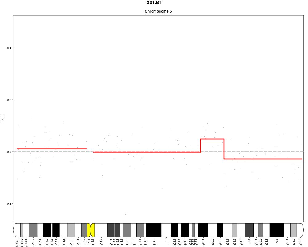
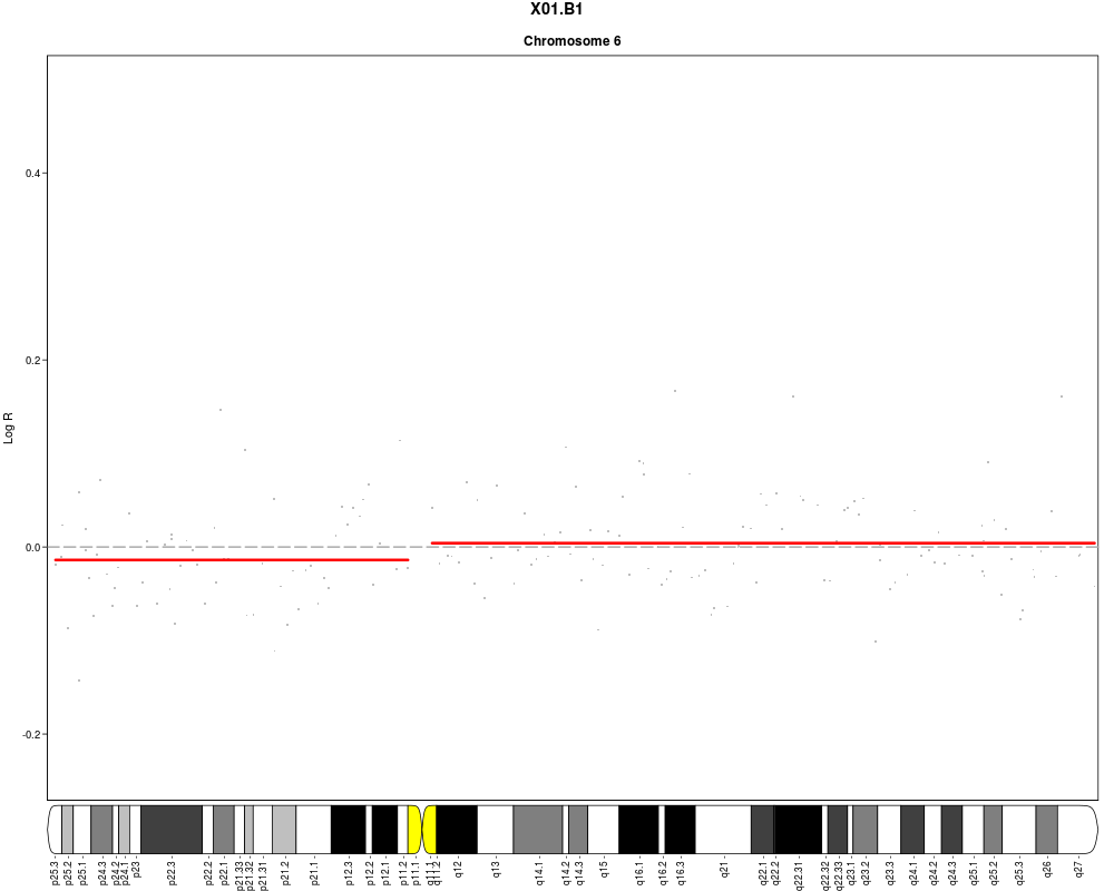
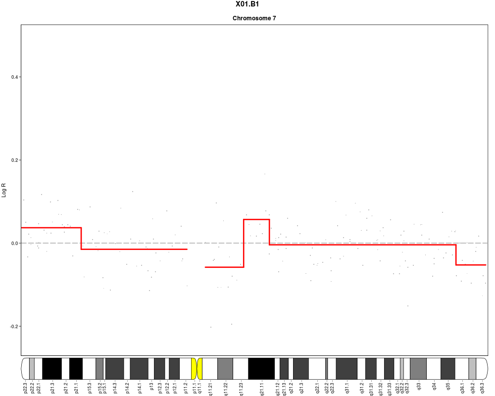
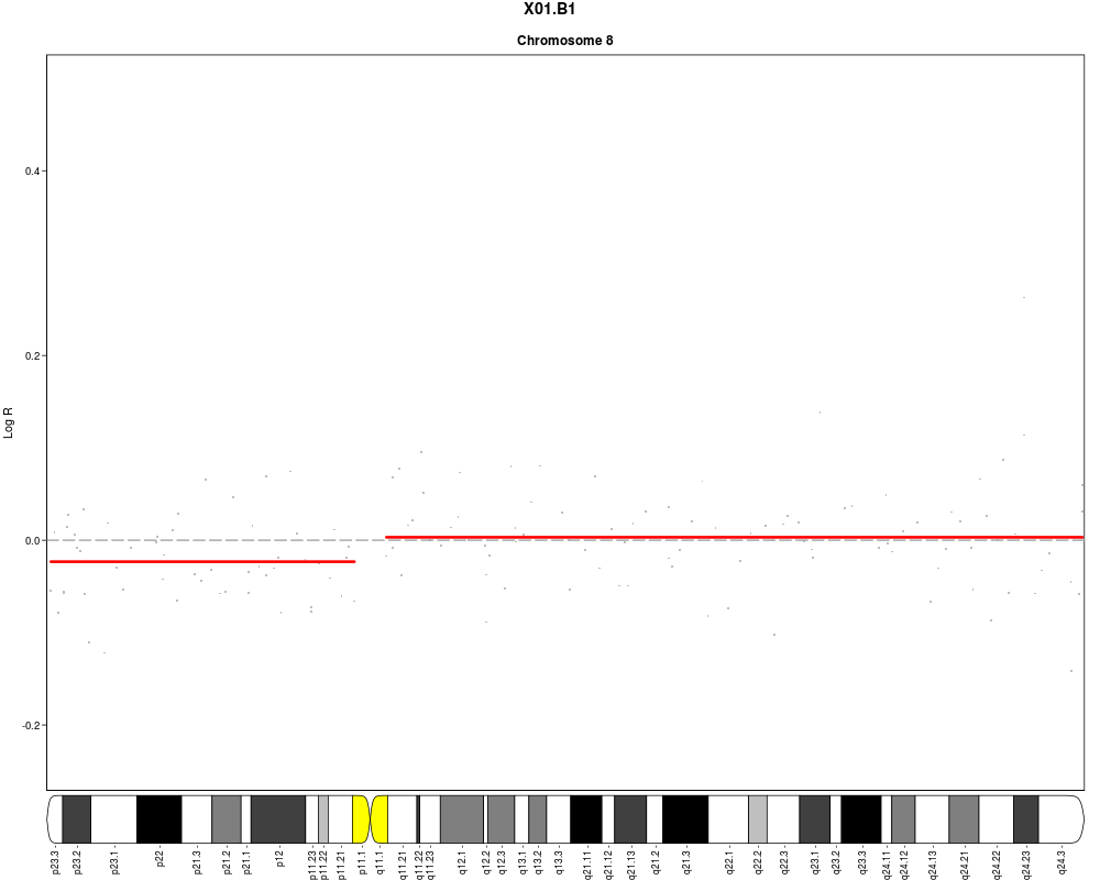
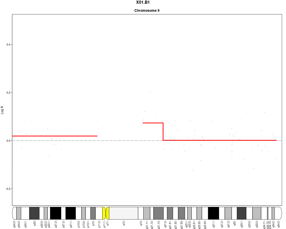
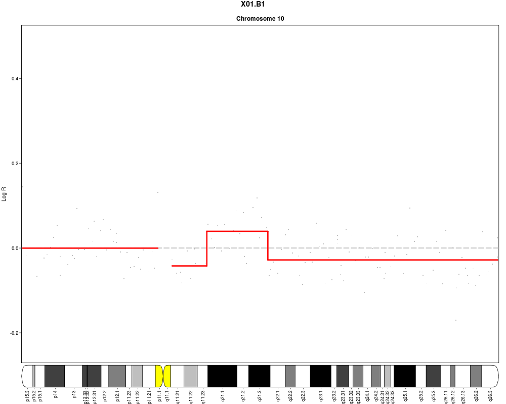
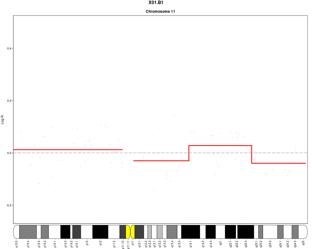
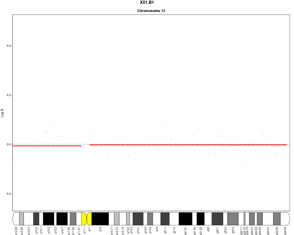
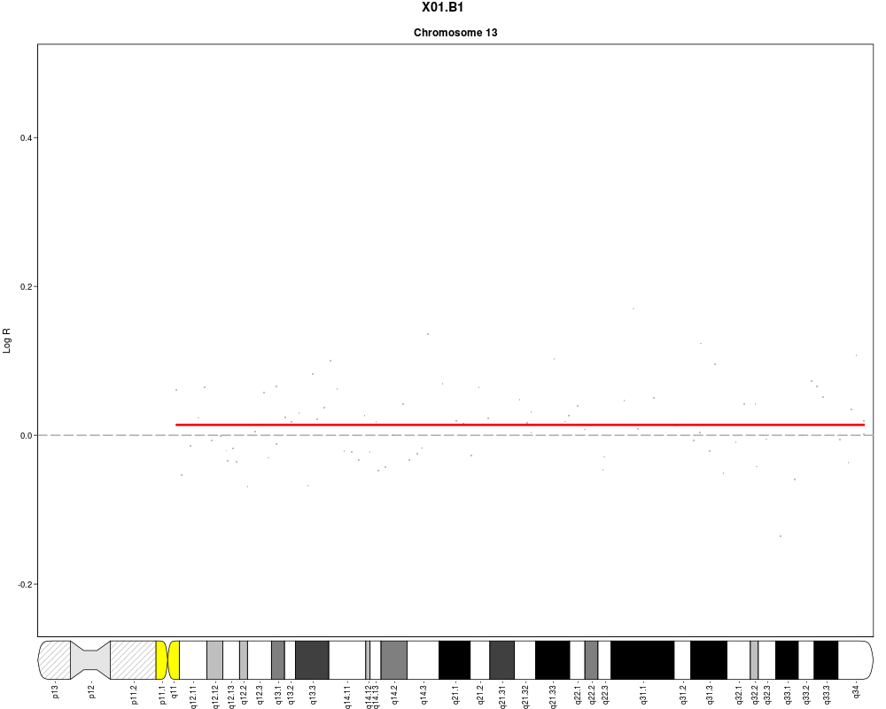
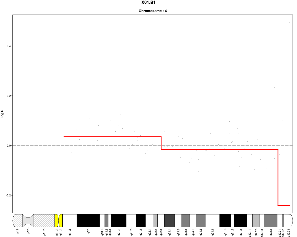
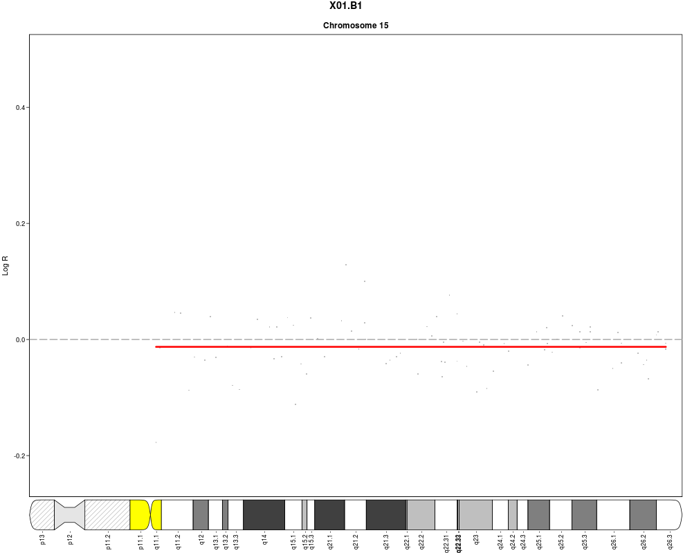
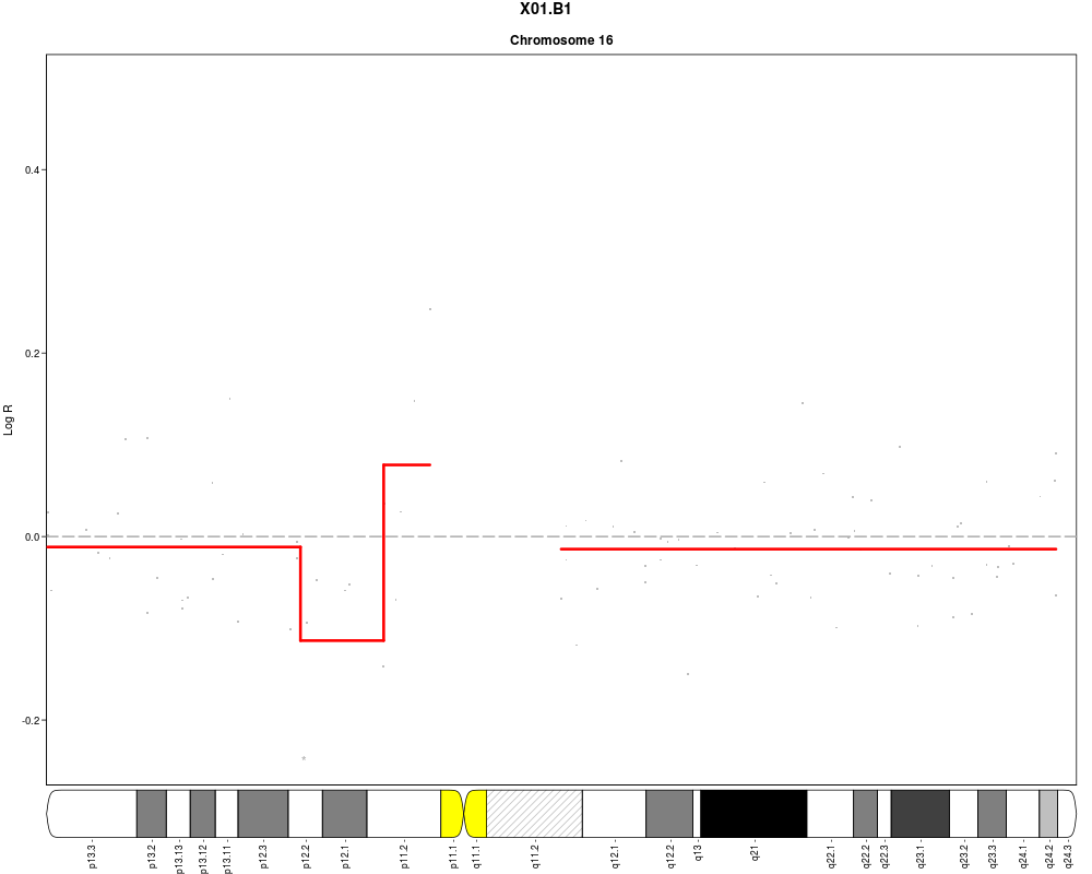
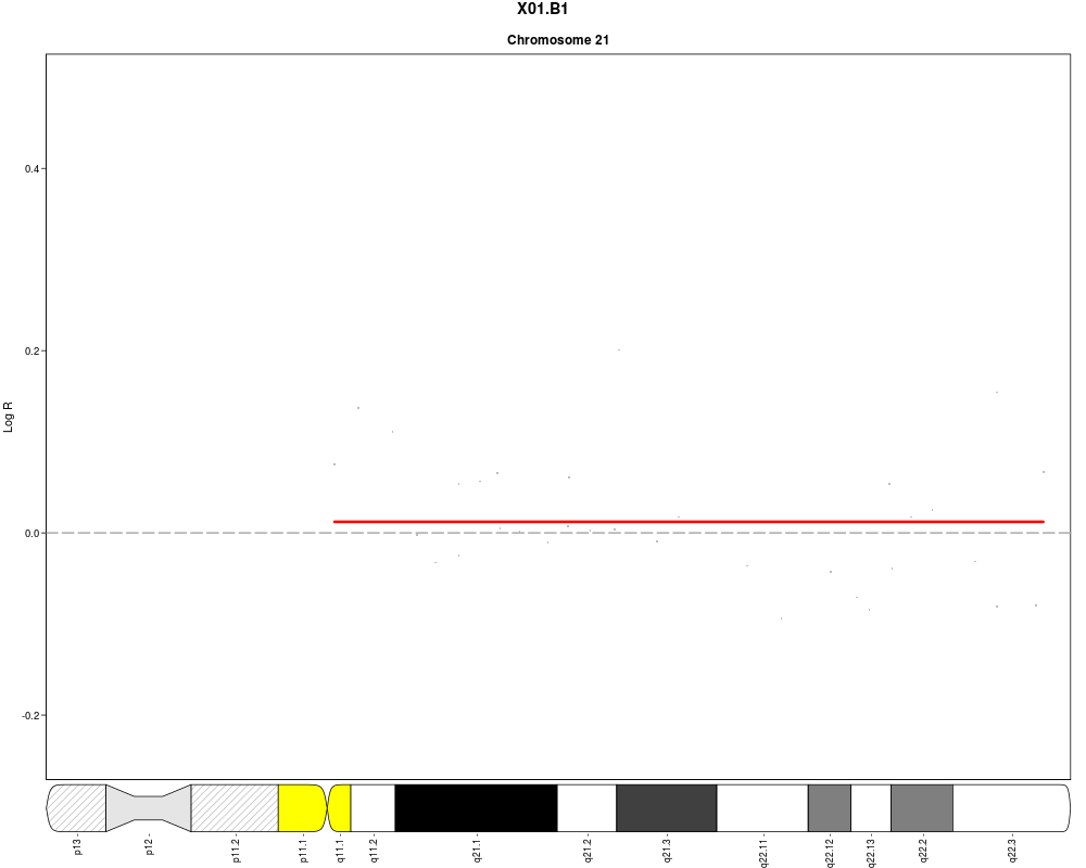
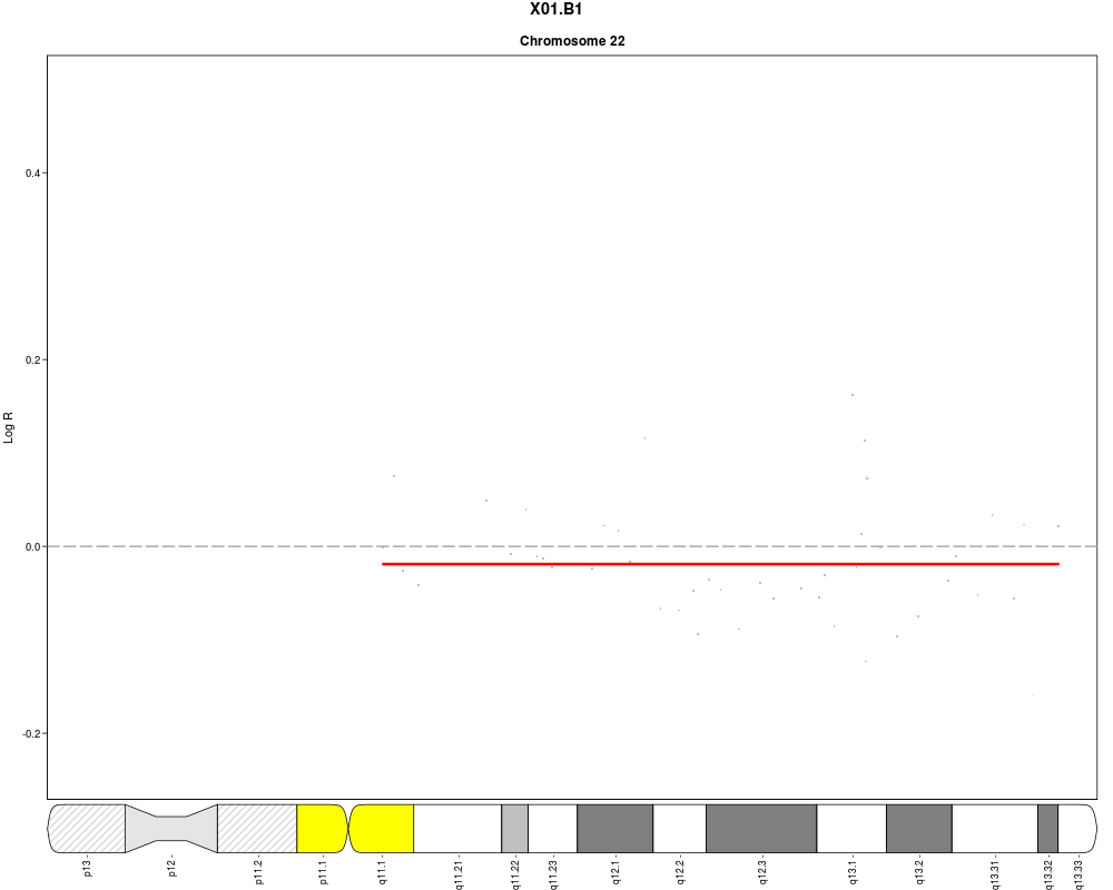
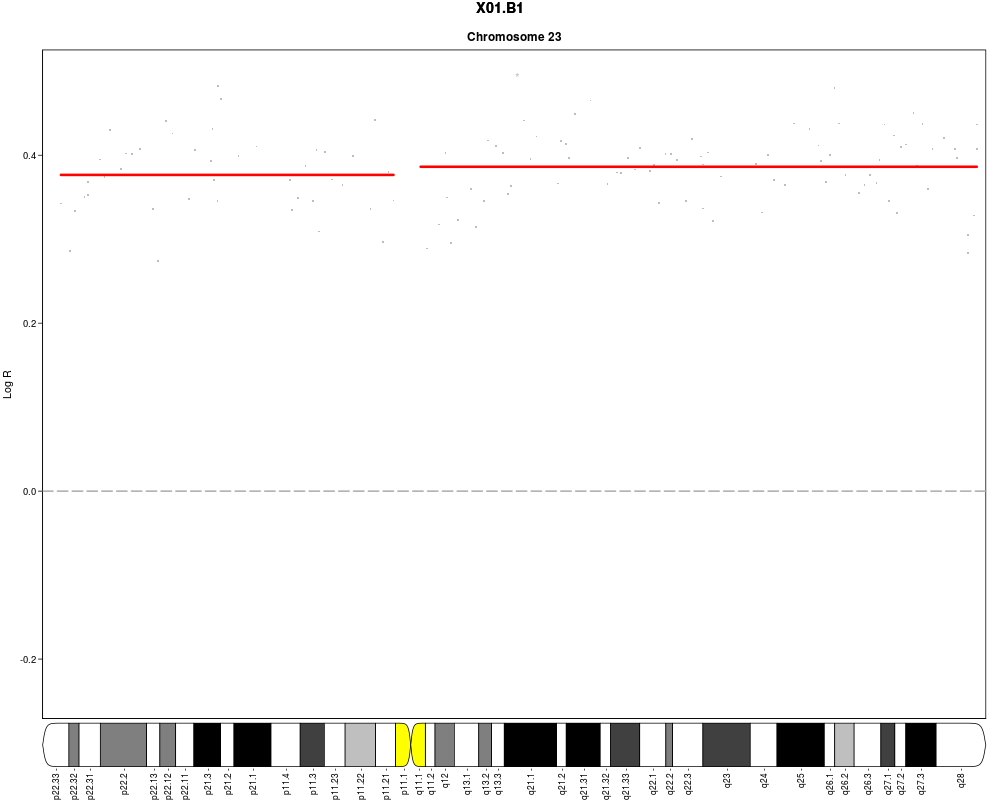
#Add cytoband text to ideogram (one page per chromosome to ensure sufficient
#space)
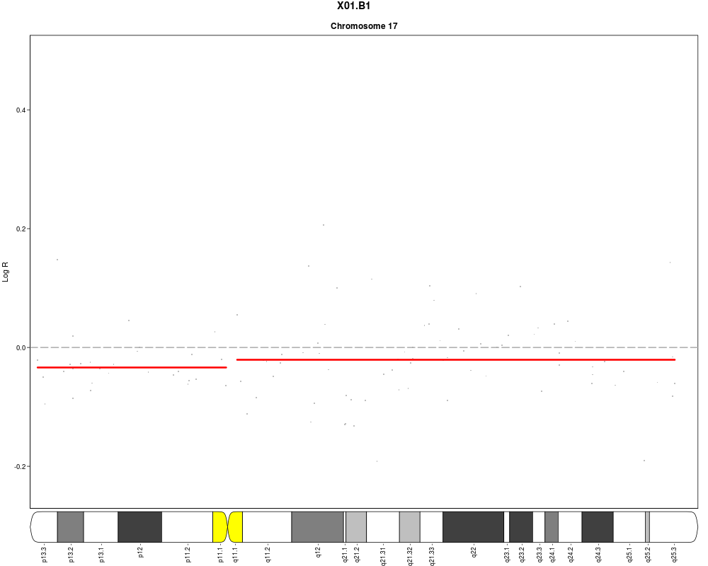
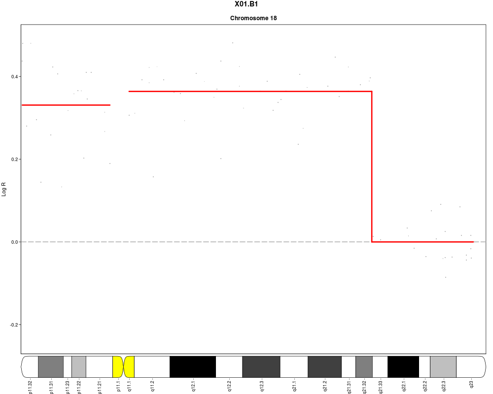
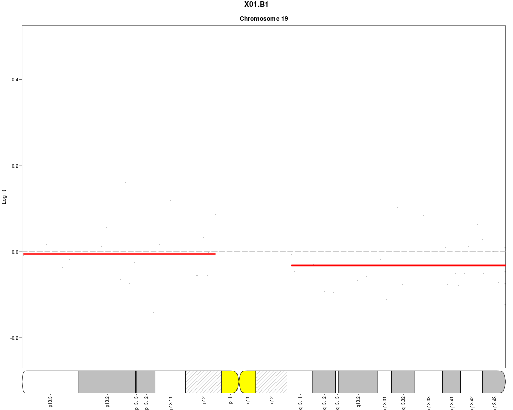
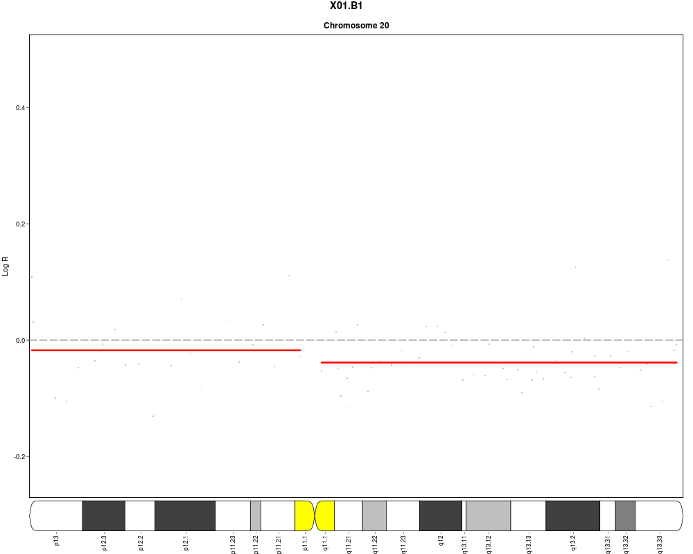
plotSample(data=sub.lymphoma,segments=uni.segments,sample=1,layout=c(1,1),
cyto.text=TRUE)
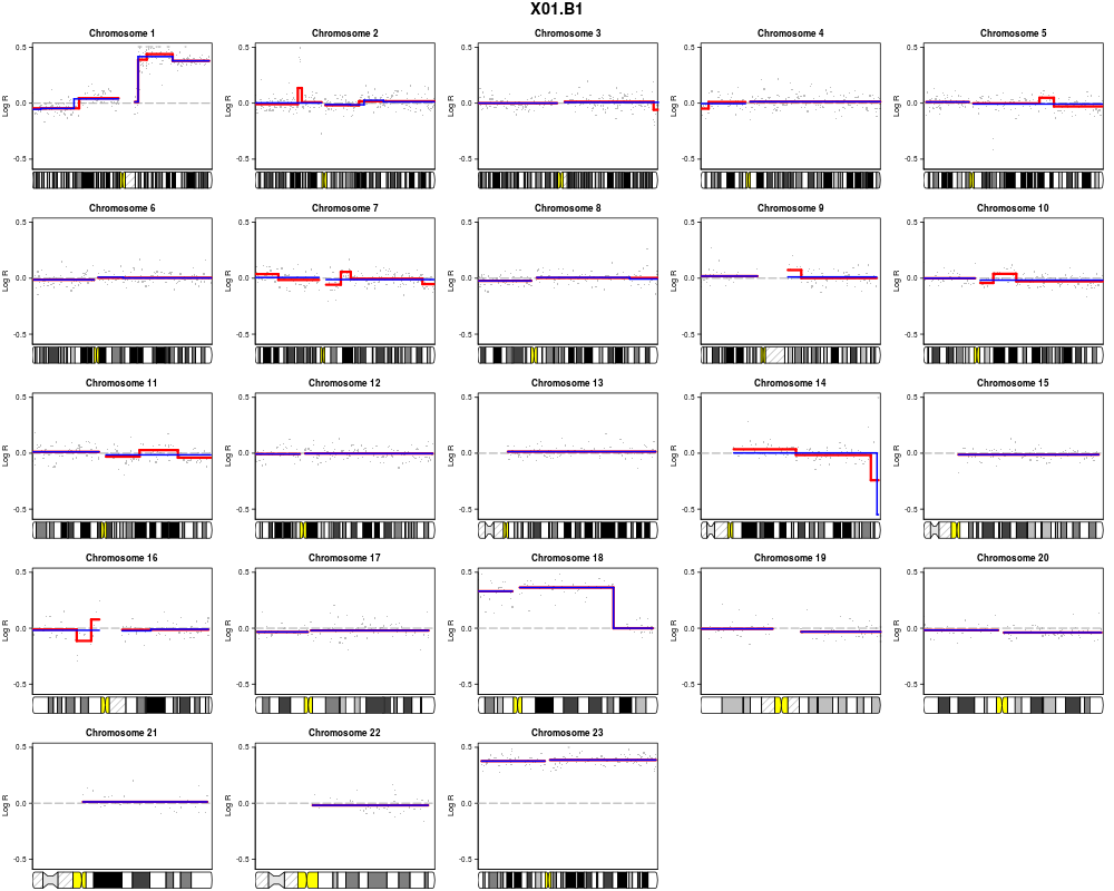
#Add multipcf-segmentation results, drop legend
plotSample(data=sub.lymphoma,segments=list(uni.segments,multi.segments),sample=1,
layout=c(5,5),seg.col=c("red","blue"),seg.lwd=c(3,2),legend=FALSE)
#Plot by chromosome for two samples, but only chromosome 1-9. One window per
#sample:
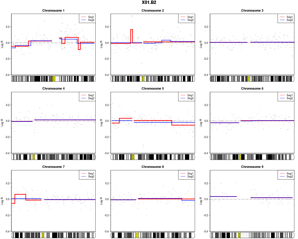
plotSample(data=sub.lymphoma,segments=list(uni.segments,multi.segments),sample=
c(2,3),chrom=c(1:9),layout=c(3,3),seg.col=c("red","blue"),
seg.lwd=c(3,2),onefile=FALSE)
#Zoom in on a particular region by setting xlim:
plotSample(data=sub.lymphoma,segments=uni.segments,sample=1,chrom=1,plot.ideo=
FALSE,xlim=c(140,170))
Results
R version 3.3.1 (2016-06-21) -- "Bug in Your Hair"
Copyright (C) 2016 The R Foundation for Statistical Computing
Platform: x86_64-pc-linux-gnu (64-bit)

R is free software and comes with ABSOLUTELY NO WARRANTY.
You are welcome to redistribute it under certain conditions.
Type 'license()' or 'licence()' for distribution details.

R is a collaborative project with many contributors.
Type 'contributors()' for more information and
'citation()' on how to cite R or R packages in publications.

Type 'demo()' for some demos, 'help()' for on-line help, or
'help.start()' for an HTML browser interface to help.
Type 'q()' to quit R.

> library(copynumber)
Loading required package: BiocGenerics
Loading required package: parallel

Attaching package: 'BiocGenerics'

The following objects are masked from 'package:parallel':

    clusterApply, clusterApplyLB, clusterCall, clusterEvalQ,
    clusterExport, clusterMap, parApply, parCapply, parLapply,
    parLapplyLB, parRapply, parSapply, parSapplyLB

The following objects are masked from 'package:stats':

    IQR, mad, xtabs

The following objects are masked from 'package:base':

    Filter, Find, Map, Position, Reduce, anyDuplicated, append,
    as.data.frame, cbind, colnames, do.call, duplicated, eval, evalq,
    get, grep, grepl, intersect, is.unsorted, lapply, lengths, mapply,
    match, mget, order, paste, pmax, pmax.int, pmin, pmin.int, rank,
    rbind, rownames, sapply, setdiff, sort, table, tapply, union,
    unique, unsplit

> png(filename="/home/ddbj/snapshot/RGM3/R_BC/result/copynumber/plotSample.Rd_%03d_medium.png", width=480, height=480)
> ### Name: plotSample
> ### Title: Plot copy number data and/or segmentation results by sample
> ### Aliases: plotSample
>
> ### ** Examples
>
> #Lymphoma data
> data(lymphoma)
> #Take out a smaller subset of 6 samples (using subsetData):
> sub.lymphoma <- subsetData(lymphoma,sample=1:6)
>
> #Winsorize data:
> wins.data <- winsorize(data=sub.lymphoma)
winsorize finished for chromosome arm 1p
winsorize finished for chromosome arm 1q
winsorize finished for chromosome arm 2p
winsorize finished for chromosome arm 2q
winsorize finished for chromosome arm 3p
winsorize finished for chromosome arm 3q
winsorize finished for chromosome arm 4p
winsorize finished for chromosome arm 4q
winsorize finished for chromosome arm 5p
winsorize finished for chromosome arm 5q
winsorize finished for chromosome arm 6p
winsorize finished for chromosome arm 6q
winsorize finished for chromosome arm 7p
winsorize finished for chromosome arm 7q
winsorize finished for chromosome arm 8p
winsorize finished for chromosome arm 8q
winsorize finished for chromosome arm 9p
winsorize finished for chromosome arm 9q
winsorize finished for chromosome arm 10p
winsorize finished for chromosome arm 10q
winsorize finished for chromosome arm 11p
winsorize finished for chromosome arm 11q
winsorize finished for chromosome arm 12p
winsorize finished for chromosome arm 12q
winsorize finished for chromosome arm 13q
winsorize finished for chromosome arm 14q
winsorize finished for chromosome arm 15q
winsorize finished for chromosome arm 16p
winsorize finished for chromosome arm 16q
winsorize finished for chromosome arm 17p
winsorize finished for chromosome arm 17q
winsorize finished for chromosome arm 18p
winsorize finished for chromosome arm 18q
winsorize finished for chromosome arm 19p
winsorize finished for chromosome arm 19q
winsorize finished for chromosome arm 20p
winsorize finished for chromosome arm 20q
winsorize finished for chromosome arm 21q
winsorize finished for chromosome arm 22q
winsorize finished for chromosome arm 23p
winsorize finished for chromosome arm 23q
>
> #Use pcf to find segments:
> uni.segments <- pcf(data=wins.data,gamma=12)
pcf finished for chromosome arm 1p
pcf finished for chromosome arm 1q
pcf finished for chromosome arm 2p
pcf finished for chromosome arm 2q
pcf finished for chromosome arm 3p
pcf finished for chromosome arm 3q
pcf finished for chromosome arm 4p
pcf finished for chromosome arm 4q
pcf finished for chromosome arm 5p
pcf finished for chromosome arm 5q
pcf finished for chromosome arm 6p
pcf finished for chromosome arm 6q
pcf finished for chromosome arm 7p
pcf finished for chromosome arm 7q
pcf finished for chromosome arm 8p
pcf finished for chromosome arm 8q
pcf finished for chromosome arm 9p
pcf finished for chromosome arm 9q
pcf finished for chromosome arm 10p
pcf finished for chromosome arm 10q
pcf finished for chromosome arm 11p
pcf finished for chromosome arm 11q
pcf finished for chromosome arm 12p
pcf finished for chromosome arm 12q
pcf finished for chromosome arm 13q
pcf finished for chromosome arm 14q
pcf finished for chromosome arm 15q
pcf finished for chromosome arm 16p
pcf finished for chromosome arm 16q
pcf finished for chromosome arm 17p
pcf finished for chromosome arm 17q
pcf finished for chromosome arm 18p
pcf finished for chromosome arm 18q
pcf finished for chromosome arm 19p
pcf finished for chromosome arm 19q
pcf finished for chromosome arm 20p
pcf finished for chromosome arm 20q
pcf finished for chromosome arm 21q
pcf finished for chromosome arm 22q
pcf finished for chromosome arm 23p
pcf finished for chromosome arm 23q
>
> #Use multipcf to find segments as well:
> multi.segments <- multipcf(data=wins.data,gamma=12)
multipcf finished for chromosome arm 1p
multipcf finished for chromosome arm 1q
multipcf finished for chromosome arm 2p
multipcf finished for chromosome arm 2q
multipcf finished for chromosome arm 3p
multipcf finished for chromosome arm 3q
multipcf finished for chromosome arm 4p
multipcf finished for chromosome arm 4q
multipcf finished for chromosome arm 5p
multipcf finished for chromosome arm 5q
multipcf finished for chromosome arm 6p
multipcf finished for chromosome arm 6q
multipcf finished for chromosome arm 7p
multipcf finished for chromosome arm 7q
multipcf finished for chromosome arm 8p
multipcf finished for chromosome arm 8q
multipcf finished for chromosome arm 9p
multipcf finished for chromosome arm 9q
multipcf finished for chromosome arm 10p
multipcf finished for chromosome arm 10q
multipcf finished for chromosome arm 11p
multipcf finished for chromosome arm 11q
multipcf finished for chromosome arm 12p
multipcf finished for chromosome arm 12q
multipcf finished for chromosome arm 13q
multipcf finished for chromosome arm 14q
multipcf finished for chromosome arm 15q
multipcf finished for chromosome arm 16p
multipcf finished for chromosome arm 16q
multipcf finished for chromosome arm 17p
multipcf finished for chromosome arm 17q
multipcf finished for chromosome arm 18p
multipcf finished for chromosome arm 18q
multipcf finished for chromosome arm 19p
multipcf finished for chromosome arm 19q
multipcf finished for chromosome arm 20p
multipcf finished for chromosome arm 20q
multipcf finished for chromosome arm 21q
multipcf finished for chromosome arm 22q
multipcf finished for chromosome arm 23p
multipcf finished for chromosome arm 23q
>
> #Plot data and pcf-segments for one sample separately for each chromosome:
> plotSample(data=sub.lymphoma,segments=uni.segments,sample=1,layout=c(5,5))
> #Add cytoband text to ideogram (one page per chromosome to ensure sufficient
> #space)
> plotSample(data=sub.lymphoma,segments=uni.segments,sample=1,layout=c(1,1),
+     cyto.text=TRUE)
> #Add multipcf-segmentation results, drop legend
> plotSample(data=sub.lymphoma,segments=list(uni.segments,multi.segments),sample=1,
+     layout=c(5,5),seg.col=c("red","blue"),seg.lwd=c(3,2),legend=FALSE)
> #Plot by chromosome for two samples, but only chromosome 1-9. One window per
> #sample:
> plotSample(data=sub.lymphoma,segments=list(uni.segments,multi.segments),sample=
+     c(2,3),chrom=c(1:9),layout=c(3,3),seg.col=c("red","blue"),
+     seg.lwd=c(3,2),onefile=FALSE)
Error in dev.new(width = arg$plot.size[1], height = arg$plot.size[2],  :
  no suitable unused file name for pdf()
Calls: plotSample -> dev.new
Execution halted
|