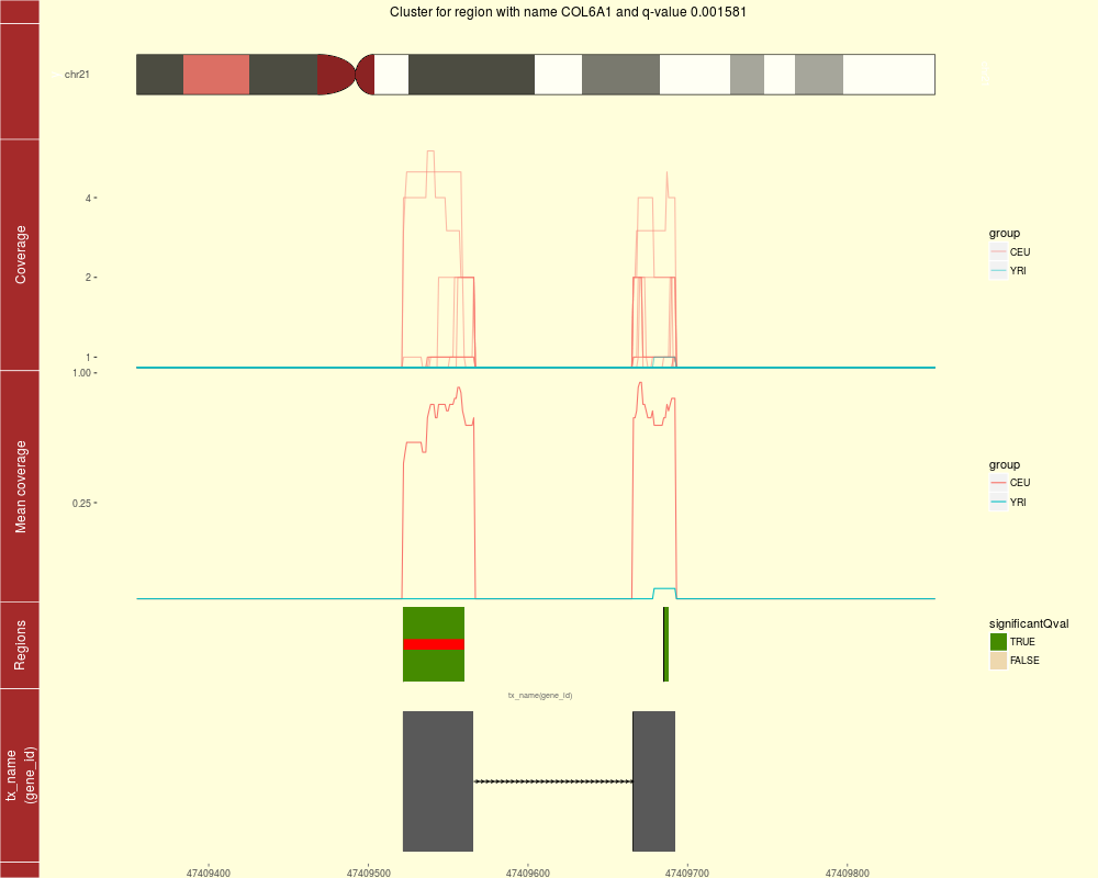
Plot the coverage information surrounding a region cluster

Description

For a given region found in calculatePvalues, plot the coverage for the cluster this region belongs to as well as some padding. The mean by group is shown to facilitate comparisons between groups. If annotation exists, you can plot the trancripts and exons (if any) overlapping in the vicinity of the region of interest.

Usage

plotCluster(idx, regions, annotation, coverageInfo, groupInfo,
  titleUse = "qval", txdb = NULL, p.ideogram = NULL, ...)

Arguments

Details

See the parameter significantCut in calculatePvalues for how the significance cutoffs are determined.

Value

A ggplot2 plot that is ready to be printed out. Tecnically it is a ggbio object. The region with the red bar is the one whose information is shown in the title.

Author(s)

Leonardo Collado-Torres

See Also

loadCoverage, calculatePvalues, annotateNearest, plotIdeogram

Examples

## Load data
library('derfinder')

## Annotate the results with bumphunter::matchGenes()
library('bumphunter')
library('TxDb.Hsapiens.UCSC.hg19.knownGene')
library('org.Hs.eg.db')
genes <- annotateTranscripts(txdb = TxDb.Hsapiens.UCSC.hg19.knownGene,
    annotationPackage = 'org.Hs.eg.db')
annotation <- matchGenes(x = genomeRegions$regions, subject = genes)

## Make the plot
plotCluster(idx=1, regions=genomeRegions$regions, annotation=annotation,
    coverageInfo=genomeDataRaw$coverage, groupInfo=genomeInfo$pop,
    txdb=TxDb.Hsapiens.UCSC.hg19.knownGene)
## Resize the plot window and the labels will look good.

## Not run: 
## For a custom plot, check the ggbio and ggplot2 packages.
## Also feel free to look at the code for this function:
plotCluster


## End(Not run)

Results

R version 3.3.1 (2016-06-21) -- "Bug in Your Hair"
Copyright (C) 2016 The R Foundation for Statistical Computing
Platform: x86_64-pc-linux-gnu (64-bit)

R is free software and comes with ABSOLUTELY NO WARRANTY.
You are welcome to redistribute it under certain conditions.
Type 'license()' or 'licence()' for distribution details.

R is a collaborative project with many contributors.
Type 'contributors()' for more information and
'citation()' on how to cite R or R packages in publications.

Type 'demo()' for some demos, 'help()' for on-line help, or
'help.start()' for an HTML browser interface to help.
Type 'q()' to quit R.

> library(derfinderPlot)
Warning message:
replacing previous import 'ggplot2::Position' by 'BiocGenerics::Position' when loading 'ggbio' 
> png(filename="/home/ddbj/snapshot/RGM3/R_BC/result/derfinderPlot/plotCluster.Rd_%03d_medium.png", width=480, height=480)
> ### Name: plotCluster
> ### Title: Plot the coverage information surrounding a region cluster
> ### Aliases: plotCluster
> 
> ### ** Examples
> 
> ## Load data
> library('derfinder')
> 
> ## Annotate the results with bumphunter::matchGenes()
> library('bumphunter')
Loading required package: S4Vectors
Loading required package: stats4
Loading required package: BiocGenerics
Loading required package: parallel

Attaching package: 'BiocGenerics'

The following objects are masked from 'package:parallel':

    clusterApply, clusterApplyLB, clusterCall, clusterEvalQ,
    clusterExport, clusterMap, parApply, parCapply, parLapply,
    parLapplyLB, parRapply, parSapply, parSapplyLB

The following objects are masked from 'package:stats':

    IQR, mad, xtabs

The following objects are masked from 'package:base':

    Filter, Find, Map, Position, Reduce, anyDuplicated, append,
    as.data.frame, cbind, colnames, do.call, duplicated, eval, evalq,
    get, grep, grepl, intersect, is.unsorted, lapply, lengths, mapply,
    match, mget, order, paste, pmax, pmax.int, pmin, pmin.int, rank,
    rbind, rownames, sapply, setdiff, sort, table, tapply, union,
    unique, unsplit


Attaching package: 'S4Vectors'

The following objects are masked from 'package:base':

    colMeans, colSums, expand.grid, rowMeans, rowSums

Loading required package: IRanges
Loading required package: GenomeInfoDb
Loading required package: GenomicRanges
Loading required package: foreach
Loading required package: iterators
Loading required package: locfit
locfit 1.5-9.1 	 2013-03-22
> library('TxDb.Hsapiens.UCSC.hg19.knownGene')
Loading required package: GenomicFeatures
Loading required package: AnnotationDbi
Loading required package: Biobase
Welcome to Bioconductor

    Vignettes contain introductory material; view with
    'browseVignettes()'. To cite Bioconductor, see
    'citation("Biobase")', and for packages 'citation("pkgname")'.

> library('org.Hs.eg.db')

> genes <- annotateTranscripts(txdb = TxDb.Hsapiens.UCSC.hg19.knownGene,
+     annotationPackage = 'org.Hs.eg.db')
Getting TSS and TSE.
Getting CSS and CSE.
Getting exons.
Annotating genes.
> annotation <- matchGenes(x = genomeRegions$regions, subject = genes)
> 
> ## Make the plot
> plotCluster(idx=1, regions=genomeRegions$regions, annotation=annotation,
+     coverageInfo=genomeDataRaw$coverage, groupInfo=genomeInfo$pop,
+     txdb=TxDb.Hsapiens.UCSC.hg19.knownGene)
Parsing transcripts...
Parsing exons...
Parsing cds...
Parsing utrs...
------exons...
------cdss...
------introns...
------utr...
aggregating...
Done
"gap" not in any of the valid gene feature terms "cds", "exon", "utr"
Constructing graphics...
> ## Resize the plot window and the labels will look good.
> 
> ## Not run: 
> ##D ## For a custom plot, check the ggbio and ggplot2 packages.
> ##D ## Also feel free to look at the code for this function:
> ##D plotCluster
> ##D 
> ## End(Not run)
> 
> 
> 
> 
> 
> dev.off()
null device 
          1 
>