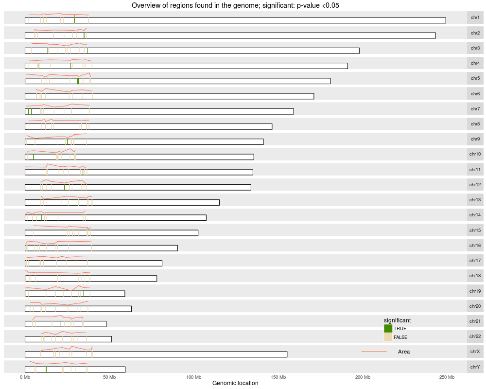
Plot a karyotype overview of the genome with the identified regions

Description

Plots an overview of the genomic locations of the identified regions (see calculatePvalues) in a karyotype view. The coloring can be done either by significant regions according to their p-values, significant by adjusted p-values, or by annotated region if using annotateNearest.

Usage

plotOverview(regions, annotation = NULL, type = "pval",
  significantCut = c(0.05, 0.1), ...)

Arguments

Value

A ggplot2 plot that is ready to be printed out. Tecnically it is a ggbio object.

Author(s)

Leonardo Collado-Torres

See Also

calculatePvalues, annotateNearest

Examples

## Construct toy data
chrs <- paste0('chr', c(1:22, 'X', 'Y'))
chrs <- factor(chrs, levels=chrs)
library('GenomicRanges')
regs <- GRanges(rep(chrs, 10), ranges=IRanges(runif(240, 1, 4e7),
    width=1e3), significant=sample(c(TRUE, FALSE), 240, TRUE, p=c(0.05,
    0.95)), significantQval=sample(c(TRUE, FALSE), 240, TRUE, p=c(0.1,
    0.9)), area=rnorm(240))
annotation <- data.frame(region=sample(c('upstream', 'promoter',
    "overlaps 5'", 'inside', "overlaps 3'", "close to 3'", 'downstream'),
    240, TRUE))

## Type pval
plotOverview(regs)

## Not run: 
## Type qval
plotOverview(regs, type='qval')

## Annotation
plotOverview(regs, annotation, type='annotation')

## Resize the plots if needed.

## You might prefer to leave the legend at ggplot2's default option: right
plotOverview(regs, legend.position='right')

## Although the legend looks better on the bottom
plotOverview(regs, legend.position='bottom')

## Example knitr chunk for higher res plot using the CairoPNG device
```{r overview, message=FALSE, fig.width=7, fig.height=9, dev='CairoPNG', dpi=300}
plotOverview(regs, base_size=30, areaRel=10, legend.position=c(0.95, 0.12))
```

## For more custom plots, take a look at the ggplot2 and ggbio packages
## and feel free to look at the code of this function:
plotOverview

## End(Not run)

Results

R version 3.3.1 (2016-06-21) -- "Bug in Your Hair"
Copyright (C) 2016 The R Foundation for Statistical Computing
Platform: x86_64-pc-linux-gnu (64-bit)

R is free software and comes with ABSOLUTELY NO WARRANTY.
You are welcome to redistribute it under certain conditions.
Type 'license()' or 'licence()' for distribution details.

R is a collaborative project with many contributors.
Type 'contributors()' for more information and
'citation()' on how to cite R or R packages in publications.

Type 'demo()' for some demos, 'help()' for on-line help, or
'help.start()' for an HTML browser interface to help.
Type 'q()' to quit R.

> library(derfinderPlot)
Warning message:
replacing previous import 'ggplot2::Position' by 'BiocGenerics::Position' when loading 'ggbio' 
> png(filename="/home/ddbj/snapshot/RGM3/R_BC/result/derfinderPlot/plotOverview.Rd_%03d_medium.png", width=480, height=480)
> ### Name: plotOverview
> ### Title: Plot a karyotype overview of the genome with the identified
> ###   regions
> ### Aliases: plotOverview
> 
> ### ** Examples
> 
> ## Construct toy data
> chrs <- paste0('chr', c(1:22, 'X', 'Y'))
> chrs <- factor(chrs, levels=chrs)
> library('GenomicRanges')
Loading required package: BiocGenerics
Loading required package: parallel

Attaching package: 'BiocGenerics'

The following objects are masked from 'package:parallel':

    clusterApply, clusterApplyLB, clusterCall, clusterEvalQ,
    clusterExport, clusterMap, parApply, parCapply, parLapply,
    parLapplyLB, parRapply, parSapply, parSapplyLB

The following objects are masked from 'package:stats':

    IQR, mad, xtabs

The following objects are masked from 'package:base':

    Filter, Find, Map, Position, Reduce, anyDuplicated, append,
    as.data.frame, cbind, colnames, do.call, duplicated, eval, evalq,
    get, grep, grepl, intersect, is.unsorted, lapply, lengths, mapply,
    match, mget, order, paste, pmax, pmax.int, pmin, pmin.int, rank,
    rbind, rownames, sapply, setdiff, sort, table, tapply, union,
    unique, unsplit

Loading required package: S4Vectors
Loading required package: stats4

Attaching package: 'S4Vectors'

The following objects are masked from 'package:base':

    colMeans, colSums, expand.grid, rowMeans, rowSums

Loading required package: IRanges
Loading required package: GenomeInfoDb
> regs <- GRanges(rep(chrs, 10), ranges=IRanges(runif(240, 1, 4e7),
+     width=1e3), significant=sample(c(TRUE, FALSE), 240, TRUE, p=c(0.05,
+     0.95)), significantQval=sample(c(TRUE, FALSE), 240, TRUE, p=c(0.1,
+     0.9)), area=rnorm(240))
> annotation <- data.frame(region=sample(c('upstream', 'promoter',
+     "overlaps 5'", 'inside', "overlaps 3'", "close to 3'", 'downstream'),
+     240, TRUE))
> 
> ## Type pval
> plotOverview(regs)
2016-07-06 14:47:02 plotOverview: assigning chromosome lengths from hg19!!!
Scale for 'x' is already present. Adding another scale for 'x', which will
replace the existing scale.
Scale for 'x' is already present. Adding another scale for 'x', which will
replace the existing scale.
> 
> ## Not run: 
> ##D ## Type qval
> ##D plotOverview(regs, type='qval')
> ##D 
> ##D ## Annotation
> ##D plotOverview(regs, annotation, type='annotation')
> ##D 
> ##D ## Resize the plots if needed.
> ##D 
> ##D ## You might prefer to leave the legend at ggplot2's default option: right
> ##D plotOverview(regs, legend.position='right')
> ##D 
> ##D ## Although the legend looks better on the bottom
> ##D plotOverview(regs, legend.position='bottom')
> ##D 
> ##D ## Example knitr chunk for higher res plot using the CairoPNG device
> ##D ```{r overview, message=FALSE, fig.width=7, fig.height=9, dev='CairoPNG', dpi=300}
> ##D plotOverview(regs, base_size=30, areaRel=10, legend.position=c(0.95, 0.12))
> ##D ```
> ##D 
> ##D ## For more custom plots, take a look at the ggplot2 and ggbio packages
> ##D ## and feel free to look at the code of this function:
> ##D plotOverview
> ## End(Not run)
> 
> 
> 
> 
> 
> dev.off()
null device 
          1 
>