Creating Filters and Filtering Flow Cytometry Data

Description

The tmixFilter function creates a filter object which is then passed to the filter method that performs filtering on a flowFrame object. This method pair is provided to let flowClust integrate with the flowCore package.

Usage

tmixFilter(filterId="tmixFilter", parameters="", ...)

Arguments

Value

The tmixFilter function returns an object of class tmixFilter that stores all the settings required for performing the filter operations.

The filter method is defined in package flowCore and returns an object of class tmixFilterResult (or tmixFilterResultList if filter@K has a length >1) that stores the filtering results.

Note

The tmixFilter function returns an object of class tmixFilter that extends the virtual parent filter class in the flowCore package. Hence, the filter operators, namely, &, |, ! and %subset%, also work for the tmixFilter class.

If filter@K is of length 1, the filter method returns an object of class tmixFilterResult. This class extends both the multipleFilterResult class (in the flowCore package) and the flowClust class. Operations defined for the multipleFilterResult class, like %in%, Subset and split, also work for the tmixFilterResult class. Likewise, methods or functions designed to retrieve filtering (clustering) information from a flowClust object can also be applied on a tmixFilterResult object. These include criterion, ruleOutliers, ruleOutliers<-, Map, posterior, importance, uncertainty and getEstimates. Various functionalities for plotting the filtering results are also available (see the links below).

If filter@K has a length >1, the function returns an object of class tmixFilterResultList. This class extends both the flowClustList class and the multipleFilterResult class. Note that when a tmixFilterResultList object is used in place of a tmixFilterResult object, in most cases the list element corresponding to the best model will be extracted and passed to the method/function call.

Author(s)

Raphael Gottardo <raph@stat.ubc.ca>, Kenneth Lo <c.lo@stat.ubc.ca>

References

Lo, K., Brinkman, R. R. and Gottardo, R. (2008) Automated Gating of Flow Cytometry Data via Robust Model-based Clustering. Cytometry A 73, 321-332.

See Also

flowClust, summary, plot, density, hist, Subset, split, ruleOutliers, Map

Examples

### The example below largely resembles the one in the flowClust
### man page.  The main purpose here is to demonstrate how the
### entire cluster analysis can be done in a fashion highly
### integrated into flowCore.


data(rituximab)

### create a filter object
s1filter <- tmixFilter("s1", c("FSC.H", "SSC.H"), K=1)
### cluster the data using FSC.H and SSC.H
res1 <- filter(rituximab, s1filter)

### remove outliers before proceeding to the second stage
# %in% operator returns a logical vector indicating whether each
# of the observations lies inside the gate or not
rituximab2 <- rituximab[rituximab %in% res1,]
# a shorthand for the above line
rituximab2 <- rituximab[res1,]
# this can also be done using the Subset method
rituximab2 <- Subset(rituximab, res1)

### cluster the data using FL1.H and FL3.H (with 3 clusters)
s2filter <- tmixFilter("s2", c("FL1.H", "FL3.H"), K=3)
res2 <- filter(rituximab2, s2filter)

show(s2filter)
show(res2)
summary(res2)

# to demonstrate the use of the split method
split(rituximab2, res2)
split(rituximab2, res2, population=list(sc1=c(1,2), sc2=3))

# to show the cluster assignment of observations
table(Map(res2))

# to show the cluster centres (i.e., the mean parameter estimates
# transformed back to the original scale) and proportions
getEstimates(res2)

### demonstrate the use of various plotting methods
# a scatterplot
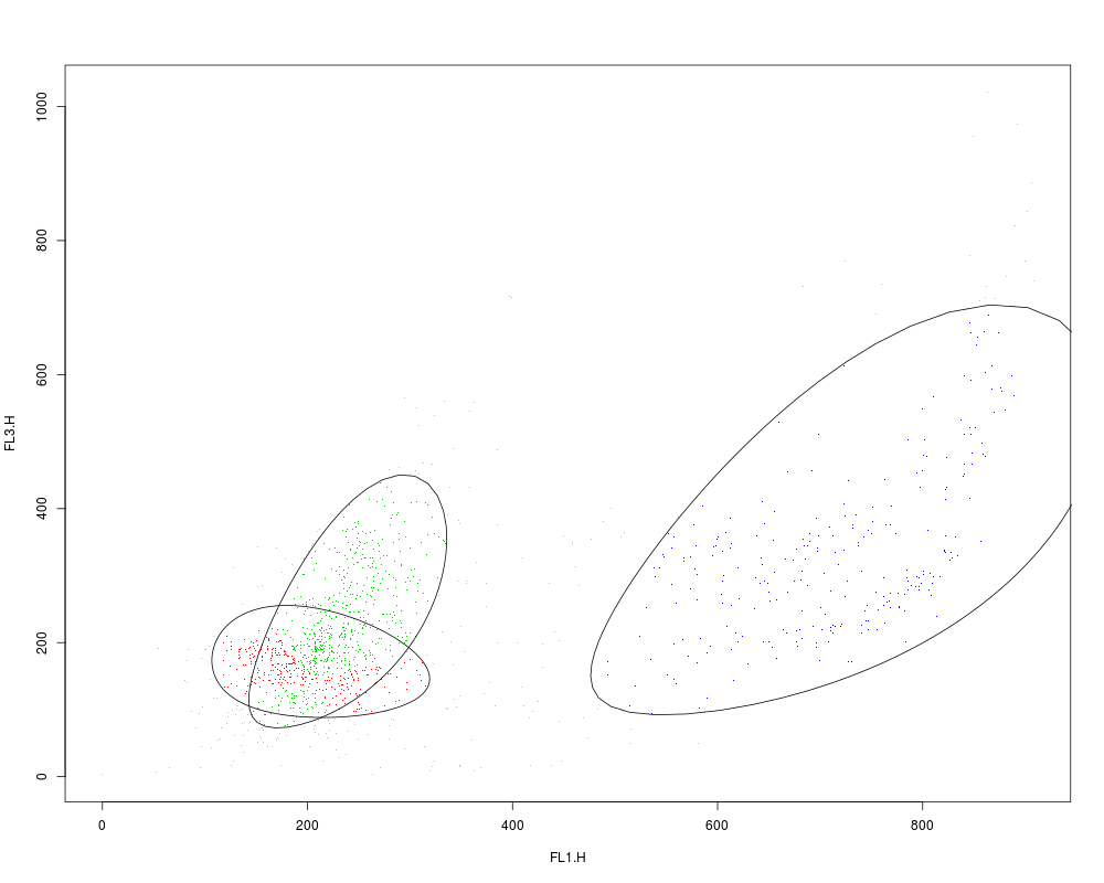
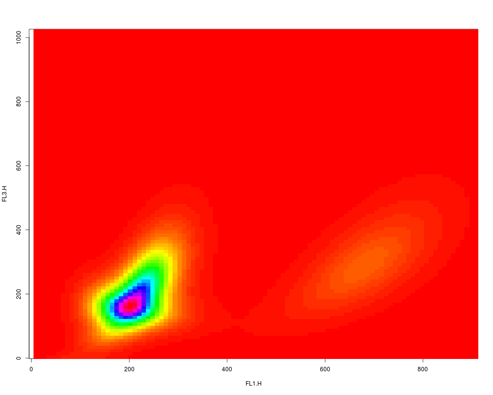
plot(rituximab2, res2, level=0.8)
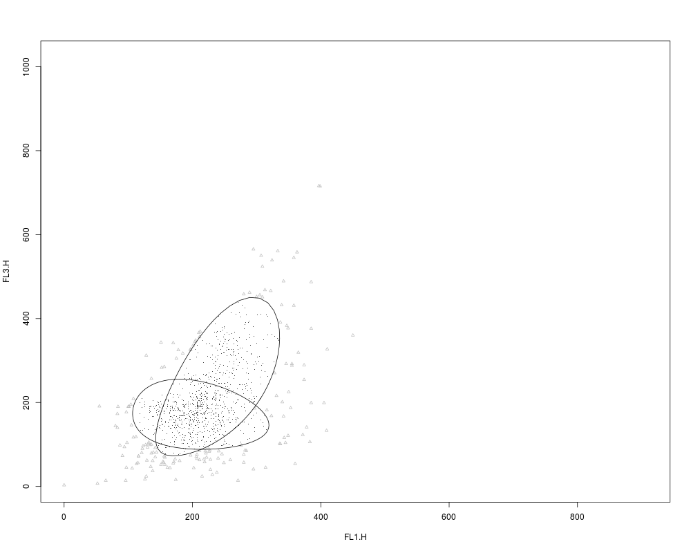
plot(rituximab2, res2, level=0.8, include=c(1,2), grayscale=TRUE,
    pch.outliers=2)
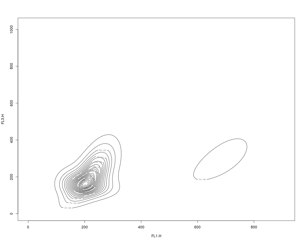
# a contour / image plot
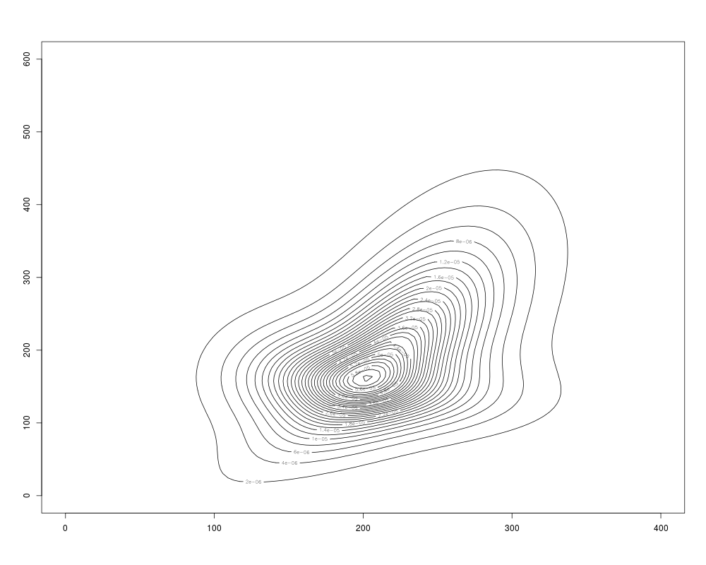
res2.den <- density(res2, data=rituximab2)
plot(res2.den)
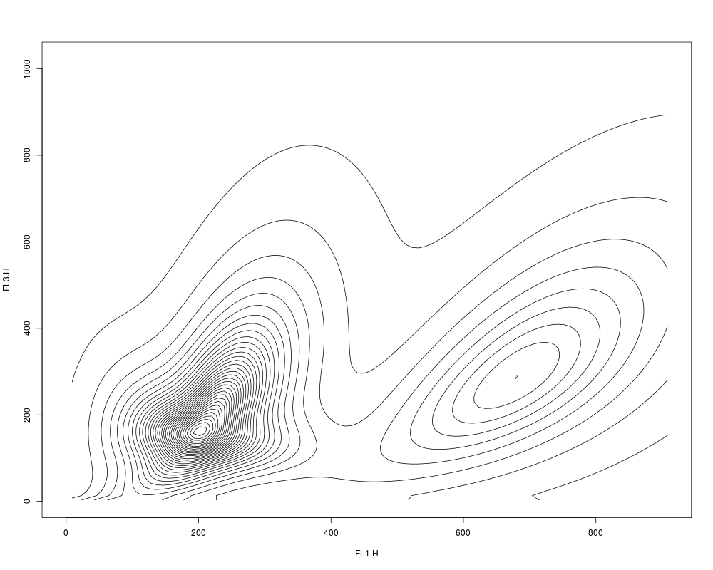
plot(res2.den, scale="sqrt", drawlabels=FALSE)
plot(res2.den, type="image", nlevels=100)
plot(density(res2, include=c(1,2), from=c(0,0), to=c(400,600)))
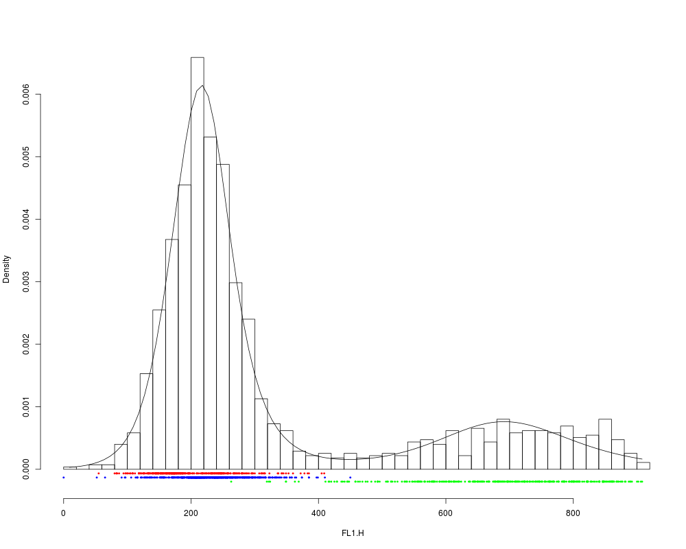
# a histogram (1-D density) plot
plot(rituximab2, res2, "FL1.H")

### to demonstrate the use of the ruleOutliers method
summary(res2)
# change the rule to call outliers
ruleOutliers(res2) <- list(level=0.95)
# augmented cluster boundaries lead to fewer outliers
summary(res2)

# the following line illustrates how to select a subset of data 
# to perform cluster analysis through the min and max arguments;
# also note the use of level to specify a rule to call outliers
# other than the default
s2t <- tmixFilter("s2t", c("FL1.H", "FL3.H"), K=3, B=100, 
    min=c(0,0), max=c(400,800), level=0.95, z.cutoff=0.5)
filter(rituximab2, s2t)

Results

R version 3.3.1 (2016-06-21) -- "Bug in Your Hair"
Copyright (C) 2016 The R Foundation for Statistical Computing
Platform: x86_64-pc-linux-gnu (64-bit)

R is free software and comes with ABSOLUTELY NO WARRANTY.
You are welcome to redistribute it under certain conditions.
Type 'license()' or 'licence()' for distribution details.

R is a collaborative project with many contributors.
Type 'contributors()' for more information and
'citation()' on how to cite R or R packages in publications.

Type 'demo()' for some demos, 'help()' for on-line help, or
'help.start()' for an HTML browser interface to help.
Type 'q()' to quit R.

> library(flowClust)
Loading required package: Biobase
Loading required package: BiocGenerics
Loading required package: parallel

Attaching package: 'BiocGenerics'

The following objects are masked from 'package:parallel':

    clusterApply, clusterApplyLB, clusterCall, clusterEvalQ,
    clusterExport, clusterMap, parApply, parCapply, parLapply,
    parLapplyLB, parRapply, parSapply, parSapplyLB

The following objects are masked from 'package:stats':

    IQR, mad, xtabs

The following objects are masked from 'package:base':

    Filter, Find, Map, Position, Reduce, anyDuplicated, append,
    as.data.frame, cbind, colnames, do.call, duplicated, eval, evalq,
    get, grep, grepl, intersect, is.unsorted, lapply, lengths, mapply,
    match, mget, order, paste, pmax, pmax.int, pmin, pmin.int, rank,
    rbind, rownames, sapply, setdiff, sort, table, tapply, union,
    unique, unsplit

Welcome to Bioconductor

    Vignettes contain introductory material; view with
    'browseVignettes()'. To cite Bioconductor, see
    'citation("Biobase")', and for packages 'citation("pkgname")'.

Loading required package: graph
Loading required package: RBGL
Loading required package: ellipse
Loading required package: flowViz
Loading required package: flowCore

Attaching package: 'flowCore'

The following object is masked from 'package:BiocGenerics':

    normalize

Loading required package: lattice
Loading required package: mnormt
Loading required package: corpcor
Loading required package: clue

Attaching package: 'flowClust'

The following object is masked from 'package:graphics':

    box

> png(filename="/home/ddbj/snapshot/RGM3/R_BC/result/flowClust/tmixFilter.Rd_%03d_medium.png", width=480, height=480)
> ### Name: tmixFilter
> ### Title: Creating Filters and Filtering Flow Cytometry Data
> ### Aliases: tmixFilter filter,flowFrame,tmixFilter-method
> ###   filter,flowFrame,filter-method filter,flowFrame,filterSet-method
> ###   filter,flowSet,filter-method filter,flowSet,filterSet-method
> ###   filter,flowSet,list-method filter-method filter.flowFrame filter
> ###   tmixFilter-class tmixFilterResult-class tmixFilterResultList
> ###   tmixFilterResultList-class %in%,flowFrame,tmixFilter-method
> ###   %in%,ANY,tmixFilterResult-method
> ###   %in%,flowFrame,tmixFilterResult-method
> ###   %in%,ANY,tmixFilterResultList-method
> ###   [,flowFrame,tmixFilterResult-method
> ###   [,flowFrame,tmixFilterResultList-method
> ###   [[,tmixFilterResultList,ANY-method
> ###   [,flowFrame,tmixFilterResult,ANY,ANY-method
> ###   [,flowFrame,tmixFilterResultList,ANY,ANY-method
> ### Keywords: cluster models
> 
> ### ** Examples
> 
> ### The example below largely resembles the one in the flowClust
> ### man page.  The main purpose here is to demonstrate how the
> ### entire cluster analysis can be done in a fashion highly
> ### integrated into flowCore.
> 
> 
> data(rituximab)
> 
> ### create a filter object
> s1filter <- tmixFilter("s1", c("FSC.H", "SSC.H"), K=1)
> ### cluster the data using FSC.H and SSC.H
> res1 <- filter(rituximab, s1filter)
The prior specification has no effect when usePrior=no
Using the parallel (multicore) version of flowClust with 4 cores
> 
> ### remove outliers before proceeding to the second stage
> # %in% operator returns a logical vector indicating whether each
> # of the observations lies inside the gate or not
> rituximab2 <- rituximab[rituximab %in% res1,]
> # a shorthand for the above line
> rituximab2 <- rituximab[res1,]
> # this can also be done using the Subset method
> rituximab2 <- Subset(rituximab, res1)
> 
> ### cluster the data using FL1.H and FL3.H (with 3 clusters)
> s2filter <- tmixFilter("s2", c("FL1.H", "FL3.H"), K=3)
> res2 <- filter(rituximab2, s2filter)
The prior specification has no effect when usePrior=no
Using the parallel (multicore) version of flowClust with 4 cores
> 
> show(s2filter)
A t-mixture filter named 's2': FL1.H, FL3.H 
** Clustering Settings ** 
Number of clusters: 3 
Degrees of freedom of t distribution: 4 
Maximum number of EM iterations: 500 
Transformation selection will be performed

Rule of identifying outliers: 90% quantile
> show(res2)
Object of class 'tmixFilterResult'
This object stores the result of applying a t-mixture filternamed 's2' on A02, which has an experiment name 'Flow Experiment'
The following parameters have been used in filtering:
	FL1.H, FL3.H

The 'tmixFilterResult' class extends the 'flowClust' class, which contains the following slots:
expName, varNames, K, w, mu, sigma, lambda, nu, z, u, label, uncertainty, ruleOutliers, flagOutliers, rm.min, rm.max, logLike, BIC, ICL
> summary(res2)
** Experiment Information ** 
Experiment name: Flow Experiment 
Variables used: FL1.H FL3.H 
** Clustering Summary ** 
Number of clusters: 3 
Proportions: 0.2658702 0.5091045 0.2250253 
** Transformation Parameter ** 
lambda: 0.4312673 
** Information Criteria ** 
Log likelihood: -16475.41 
BIC: -33080.88 
ICL: -34180.67 
** Data Quality ** 
Number of points filtered from above: 0 (0%)
Number of points filtered from below: 0 (0%)
Rule of identifying outliers: 90% quantile
Number of outliers: 96 (6.99%)
Uncertainty summary: 
> 
> # to demonstrate the use of the split method
> split(rituximab2, res2)
[[1]]
flowFrame object 'A02 (1)'
with 320 cells and 8 observables:
     name               desc range maxRange minRange
$P1 FSC.H         FSC-Height  1024     1023        0
$P2 SSC.H       Side Scatter  1024     1023        0
$P3 FL1.H     Anti-BrdU FITC  1024     1023        0
$P4 FL2.H               <NA>  1024     1023        0
$P5 FL3.H              7 AAD  1024     1023        0
$P6 FL1.A               <NA>  1024     1023        0
$P7 FL1.W               <NA>  1024     1023        0
$P8  Time Time (204.80 sec.)  1024     1023        0
136 keywords are stored in the 'description' slot

[[2]]
flowFrame object 'A02 (2)'
with 670 cells and 8 observables:
     name               desc range maxRange minRange
$P1 FSC.H         FSC-Height  1024     1023        0
$P2 SSC.H       Side Scatter  1024     1023        0
$P3 FL1.H     Anti-BrdU FITC  1024     1023        0
$P4 FL2.H               <NA>  1024     1023        0
$P5 FL3.H              7 AAD  1024     1023        0
$P6 FL1.A               <NA>  1024     1023        0
$P7 FL1.W               <NA>  1024     1023        0
$P8  Time Time (204.80 sec.)  1024     1023        0
136 keywords are stored in the 'description' slot

[[3]]
flowFrame object 'A02 (3)'
with 288 cells and 8 observables:
     name               desc range maxRange minRange
$P1 FSC.H         FSC-Height  1024     1023        0
$P2 SSC.H       Side Scatter  1024     1023        0
$P3 FL1.H     Anti-BrdU FITC  1024     1023        0
$P4 FL2.H               <NA>  1024     1023        0
$P5 FL3.H              7 AAD  1024     1023        0
$P6 FL1.A               <NA>  1024     1023        0
$P7 FL1.W               <NA>  1024     1023        0
$P8  Time Time (204.80 sec.)  1024     1023        0
136 keywords are stored in the 'description' slot

> split(rituximab2, res2, population=list(sc1=c(1,2), sc2=3))
$sc1
flowFrame object 'A02 (1,2)'
with 990 cells and 8 observables:
     name               desc range maxRange minRange
$P1 FSC.H         FSC-Height  1024     1023        0
$P2 SSC.H       Side Scatter  1024     1023        0
$P3 FL1.H     Anti-BrdU FITC  1024     1023        0
$P4 FL2.H               <NA>  1024     1023        0
$P5 FL3.H              7 AAD  1024     1023        0
$P6 FL1.A               <NA>  1024     1023        0
$P7 FL1.W               <NA>  1024     1023        0
$P8  Time Time (204.80 sec.)  1024     1023        0
3 keywords are stored in the 'description' slot

$sc2
flowFrame object 'A02 (3)'
with 288 cells and 8 observables:
     name               desc range maxRange minRange
$P1 FSC.H         FSC-Height  1024     1023        0
$P2 SSC.H       Side Scatter  1024     1023        0
$P3 FL1.H     Anti-BrdU FITC  1024     1023        0
$P4 FL2.H               <NA>  1024     1023        0
$P5 FL3.H              7 AAD  1024     1023        0
$P6 FL1.A               <NA>  1024     1023        0
$P7 FL1.W               <NA>  1024     1023        0
$P8  Time Time (204.80 sec.)  1024     1023        0
136 keywords are stored in the 'description' slot

> 
> # to show the cluster assignment of observations
> table(Map(res2))

  1   2   3 
320 670 288 
> 
> # to show the cluster centres (i.e., the mean parameter estimates
> # transformed back to the original scale) and proportions
> getEstimates(res2)
$proportions
[1] 0.2658702 0.5091045 0.2250253

$locations
         [,1]     [,2]
[1,] 196.7897 159.5326
[2,] 227.7338 215.6581
[3,] 699.9997 316.2946

> 
> ### demonstrate the use of various plotting methods
> # a scatterplot
> plot(rituximab2, res2, level=0.8)
Rule of identifying outliers: 80% quantile
> plot(rituximab2, res2, level=0.8, include=c(1,2), grayscale=TRUE,
+     pch.outliers=2)
Rule of identifying outliers: 80% quantile
> # a contour / image plot
> res2.den <- density(res2, data=rituximab2)
> plot(res2.den)
> plot(res2.den, scale="sqrt", drawlabels=FALSE)
> plot(res2.den, type="image", nlevels=100)
> plot(density(res2, include=c(1,2), from=c(0,0), to=c(400,600)))
> # a histogram (1-D density) plot
> plot(rituximab2, res2, "FL1.H")
> 
> ### to demonstrate the use of the ruleOutliers method
> summary(res2)
** Experiment Information ** 
Experiment name: Flow Experiment 
Variables used: FL1.H FL3.H 
** Clustering Summary ** 
Number of clusters: 3 
Proportions: 0.2658702 0.5091045 0.2250253 
** Transformation Parameter ** 
lambda: 0.4312673 
** Information Criteria ** 
Log likelihood: -16475.41 
BIC: -33080.88 
ICL: -34180.67 
** Data Quality ** 
Number of points filtered from above: 0 (0%)
Number of points filtered from below: 0 (0%)
Rule of identifying outliers: 90% quantile
Number of outliers: 96 (6.99%)
Uncertainty summary: 
> # change the rule to call outliers
> ruleOutliers(res2) <- list(level=0.95)
Rule of identifying outliers: 95% quantile
> # augmented cluster boundaries lead to fewer outliers
> summary(res2)
** Experiment Information ** 
Experiment name: Flow Experiment 
Variables used: FL1.H FL3.H 
** Clustering Summary ** 
Number of clusters: 3 
Proportions: 0.2658702 0.5091045 0.2250253 
** Transformation Parameter ** 
lambda: 0.4312673 
** Information Criteria ** 
Log likelihood: -16475.41 
BIC: -33080.88 
ICL: -34180.67 
** Data Quality ** 
Number of points filtered from above: 0 (0%)
Number of points filtered from below: 0 (0%)
Rule of identifying outliers: 95% quantile
Number of outliers: 35 (2.55%)
Uncertainty summary: 
> 
> # the following line illustrates how to select a subset of data 
> # to perform cluster analysis through the min and max arguments;
> # also note the use of level to specify a rule to call outliers
> # other than the default
> s2t <- tmixFilter("s2t", c("FL1.H", "FL3.H"), K=3, B=100, 
+     min=c(0,0), max=c(400,800), level=0.95, z.cutoff=0.5)
> filter(rituximab2, s2t)
The prior specification has no effect when usePrior=no
Using the parallel (multicore) version of flowClust with 4 cores
Object of class 'tmixFilterResult'
This object stores the result of applying a t-mixture filternamed 's2t' on A02, which has an experiment name 'Flow Experiment'
The following parameters have been used in filtering:
	FL1.H, FL3.H

The 'tmixFilterResult' class extends the 'flowClust' class, which contains the following slots:
expName, varNames, K, w, mu, sigma, lambda, nu, z, u, label, uncertainty, ruleOutliers, flagOutliers, rm.min, rm.max, logLike, BIC, ICL
> 
> 
> 
> 
> 
> dev.off()
null device 
          1 
>