R Graphical Manual

Browse All

Last data update: 2014.03.03

R: Mode estimation for continuous data

half.range.mode

R Documentation

Mode estimation for continuous data

Description

For data assumed to be drawn from a unimodal, continuous distribution, the mode is estimated by the “half-range” method. Bootstrap resampling for variance reduction may optionally be used.

Usage

half.range.mode(data, B, B.sample, beta = 0.5, diag = FALSE)

Arguments

`data`	A numeric vector of data from which to estimate the mode.
`B`	Optionally, the number of bootstrap resampling rounds to use. Note that `B = 1` resamples 1 time, whereas omitting `B` uses `data` as is, without resampling.
`B.sample`	If bootstrap resampling is requested, the size of the bootstrap samples drawn from `data`. Default is to use a sample which is the same size as `data`. For large data sets, this may be slow and unnecessary.
`beta`	The fraction of the remaining range to use at each iteration.
`diag`	Print extensive diagnostics. For internal testing only... best left `FALSE`.

Details

Briefly, the mode estimator is computed by iteratively identifying densest half ranges. (Other fractions of the current range can be requested by setting beta to something other than 0.5.) A densest half range is an interval whose width equals half the current range, and which contains the maximal number of observations. The subset of observations falling in the selected densest half range is then used to compute a new range, and the procedure is iterated. See the references for details.

If bootstrapping is requested, B half-range mode estimates are computed for B bootstrap samples, and their average is returned as the final estimate.

Value

The mode estimate.

Author(s)

Richard Bourgon <bourgon@stat.berkeley.edu>

References

DR Bickel, “Robust estimators of the mode and skewness of continuous data.” Computational Statistics & Data Analysis 39:153-163 (2002).
SB Hedges and P Shah, “Comparison of mode estimation methods and application in molecular clock analysis.” BMC Bioinformatics 4:31-41 (2003).

Examples

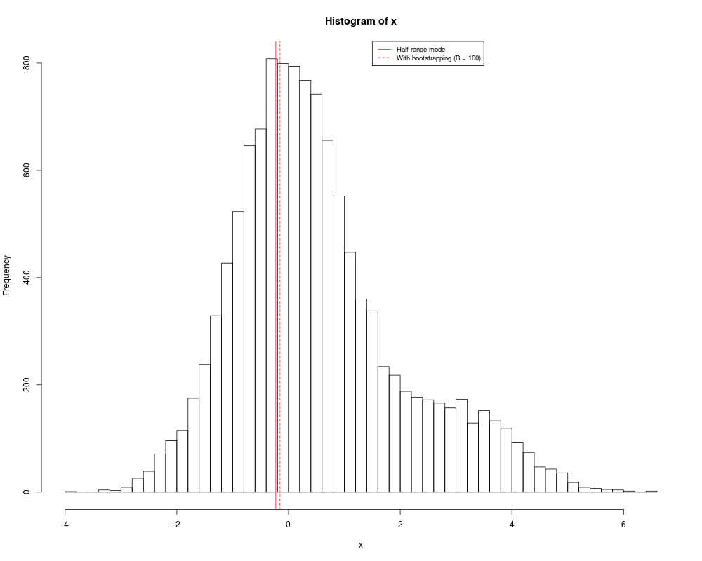
## A single normal-mixture data set

x <- c( rnorm(10000), rnorm(2000, mean = 3) )
M <- half.range.mode( x )
M.bs <- half.range.mode( x, B = 100 )

if(interactive()){
hist( x, breaks = 40 )
abline( v = c( M, M.bs ), col = "red", lty = 1:2 )
legend(
       1.5, par("usr")[4],
       c( "Half-range mode", "With bootstrapping (B = 100)" ),
       lwd = 1, lty = 1:2, cex = .8, col = "red"
       )
}

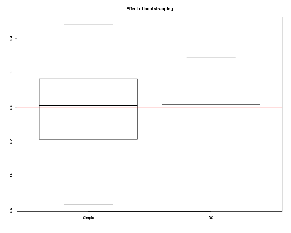
# Sampling distribution, with and without bootstrapping

X <- rbind(
           matrix( rnorm(1000 * 100), ncol = 100 ),
           matrix( rnorm(200 * 100, mean = 3), ncol = 100 )
           )
M.list <- list(
               Simple = apply( X, 2, half.range.mode ),
               BS = apply( X, 2, half.range.mode, B = 100 )
               )

if(interactive()){
boxplot( M.list, main = "Effect of bootstrapping" )
abline( h = 0, col = "red" )
}

Results


R version 3.3.1 (2016-06-21) -- "Bug in Your Hair"
Copyright (C) 2016 The R Foundation for Statistical Computing
Platform: x86_64-pc-linux-gnu (64-bit)

R is free software and comes with ABSOLUTELY NO WARRANTY.
You are welcome to redistribute it under certain conditions.
Type 'license()' or 'licence()' for distribution details.

R is a collaborative project with many contributors.
Type 'contributors()' for more information and
'citation()' on how to cite R or R packages in publications.

Type 'demo()' for some demos, 'help()' for on-line help, or
'help.start()' for an HTML browser interface to help.
Type 'q()' to quit R.

> library(genefilter)
> png(filename="/home/ddbj/snapshot/RGM3/R_BC/result/genefilter/half.range.mode.Rd_%03d_medium.png", width=480, height=480)
> ### Name: half.range.mode
> ### Title: Mode estimation for continuous data
> ### Aliases: half.range.mode
> ### Keywords: univar robust
> 
> ### ** Examples
> 
> ## A single normal-mixture data set
> 
> x <- c( rnorm(10000), rnorm(2000, mean = 3) )
> M <- half.range.mode( x )
> M.bs <- half.range.mode( x, B = 100 )
> 
> #if(interactive()){
> hist( x, breaks = 40 )
> abline( v = c( M, M.bs ), col = "red", lty = 1:2 )
> legend(
+        1.5, par("usr")[4],
+        c( "Half-range mode", "With bootstrapping (B = 100)" ),
+        lwd = 1, lty = 1:2, cex = .8, col = "red"
+        )
> #}
> 
> # Sampling distribution, with and without bootstrapping
> 
> X <- rbind(
+            matrix( rnorm(1000 * 100), ncol = 100 ),
+            matrix( rnorm(200 * 100, mean = 3), ncol = 100 )
+            )
> M.list <- list(
+                Simple = apply( X, 2, half.range.mode ),
+                BS = apply( X, 2, half.range.mode, B = 100 )
+                )
> 
> #if(interactive()){
> boxplot( M.list, main = "Effect of bootstrapping" )
> abline( h = 0, col = "red" )
> #}
> 
> 
> 
> 
> 
> dev.off()
null device 
          1 
>