R Graphical Manual

Browse All

Last data update: 2014.03.03

R: Line plot(s) for meta-region profiles

plotMeta

R Documentation

Line plot(s) for meta-region profiles

Description

Function calculates meta-profile(s) from a ScoreMatrix or a ScoreMatrixList, then produces a line plot or a set of line plots for meta-region profiles

Usage

plotMeta(mat, centralTend = "mean", overlay = TRUE, winsorize = c(0, 100),
  profile.names = NULL, xcoords = NULL, meta.rescale = FALSE,
  smoothfun = NULL, line.col = NULL, dispersion = NULL,
  dispersion.col = NULL, ylim = NULL, ylab = "average score",
  xlab = "bases", ...)

Arguments

`mat`	`ScoreMatrix` or `ScoreMatrixList` object. If it is a `ScoreMatrixList` object, all matrices in the ScoreMatrixList should have the same number of columns.
`centralTend`	a character that determines central tendency of meta-profile(s). It takes "mean" (default) or "median".
`overlay`	If TRUE multiple profiles will be overlayed in the same plot (Default:TRUE). If FALSE, and mat is a ScoreMatrixList, consider using par(mfrow=c(1,length(mat))) to see the plots from all matrices at once.
`winsorize`	Numeric vector of two, defaults to c(0,100). This vector determines the upper and lower percentile values to limit the extreme values. For example, c(0,99) will limit the values to only 99th percentile, everything above the 99 percentile will be equalized to the value of 99th percentile.This is useful for visualization of matrices that have outliers.
`profile.names`	a character vector for names of the profiles. The order should be same as the as the order of ScoreMatrixList.
`xcoords`	a numeric vector which designates relative base positions of the meta-region profiles. For example, for a 2001 column ScoreMatrix, xcoord=-1000:1000 indicates relative positions of each column in the score matrix. If NULL (Default), xcoords equals to 1:ncol(mat)
`meta.rescale`	if TRUE meta-region profiles are scaled to 0 to 1 range by subtracting the min from profiles and dividing them by max-min. If dispersion is not NULL, then dispersion will be scaled as well.
`smoothfun`	a function to smooth central tendency and dispersion bands (Default: NULL), e.g. stats::lowess.
`line.col`	color of lines for `centralTend` of meta-region profiles. Defaults to colors from `rainbow()` function.
`dispersion`	shows dispersion interval bands around `centralTend` (default:NULL). It takes one of the character: "se"shows standard error of the mean and 95 percent confidence interval for the mean "sd"shows standard deviation and 2(standard deviation) "IQR"shows 1st and 3rd quartile and confidence interval around the median based on the median +/- 1.57 IQR/sqrt(n) (notches)
`dispersion.col`	color of bands of `dispersion`. Defaults to colors from `rainbow()` and transparency is set to 0.5 (rainbow(length(mat), alpha = 0.5)).
`ylim`	same as `ylim` at `plot` function. if NULL ylim is estimated from all meta-region profiles.
`ylab`	same as `ylab` at `plot` function. Default: "average score"
`xlab`	same as `xlab` at `plot` function. Default: "bases"
`...`	other options to `plot`

Value

returns the meta-region profiles invisibly as a matrix.

Note

Score matrices are plotted according to ScoreMatrixList order. If ScoreMatrixList contains more than one matrix then they will overlap each other on a plot, i.e. the first one is plotted first and every next one overlays previous one(s) and the last one is the topmost.

Missing values in data slow down plotting dispersion around central tendency. The reason is that dispersion is plotted only for non-missing values, for each segment that contains numerical values graphics::polygon function is used to plot dispersion bands. There might be a situation, when in a column of ScoreMatrix is only one numeric number and the rest are NAs, then at corresponding position only central tendency will be plotted.

Notches show the 95 percent confidence interval for the median according to an approximation based on the normal distribution. They are used to compare groups - if notches corresponding to adjacent base pairs on the plot do not overlap, this is strong evidence that medians differ. Small sample sizes (5-10) can cause notches to extend beyond the interquartile range (IQR) (Martin Krzywinski et al. Nature Methods 11, 119-120 (2014))

Examples

data(cage)
 data(promoters)
 scores1=ScoreMatrix(target=cage,windows=promoters,strand.aware=TRUE)

 data(cpgi)
 scores2=ScoreMatrix(target=cpgi,windows=promoters,strand.aware=TRUE)

 # create a new ScoreMatrixList
 x=new("ScoreMatrixList",list(scores1,scores2))
 
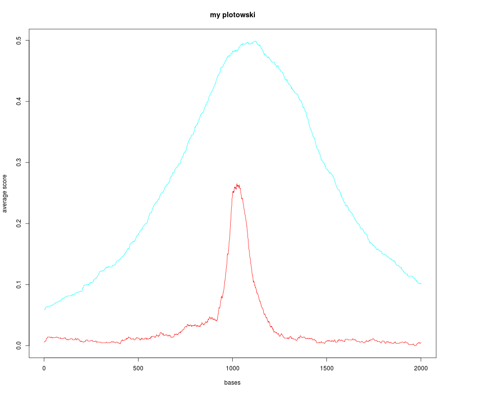
 plotMeta(mat=x,overlay=TRUE,main="my plotowski")

 # plot dispersion nd smooth central tendency and variation interval bands
 plotMeta(mat=x, centralTend="mean", dispersion="se", winsorize=c(0,99),
         main="Dispersion as interquartile band", lwd=4,
         smoothfun=function(x) stats::lowess(x, f = 1/5))

Results


R version 3.3.1 (2016-06-21) -- "Bug in Your Hair"
Copyright (C) 2016 The R Foundation for Statistical Computing
Platform: x86_64-pc-linux-gnu (64-bit)

R is free software and comes with ABSOLUTELY NO WARRANTY.
You are welcome to redistribute it under certain conditions.
Type 'license()' or 'licence()' for distribution details.

R is a collaborative project with many contributors.
Type 'contributors()' for more information and
'citation()' on how to cite R or R packages in publications.

Type 'demo()' for some demos, 'help()' for on-line help, or
'help.start()' for an HTML browser interface to help.
Type 'q()' to quit R.

> library(genomation)
Loading required package: grid
> png(filename="/home/ddbj/snapshot/RGM3/R_BC/result/genomation/plotMeta.Rd_%03d_medium.png", width=480, height=480)
> ### Name: plotMeta
> ### Title: Line plot(s) for meta-region profiles
> ### Aliases: plotMeta
> 
> ### ** Examples
> 
> data(cage)
>  data(promoters)
>  scores1=ScoreMatrix(target=cage,windows=promoters,strand.aware=TRUE)
> 
>  data(cpgi)
>  scores2=ScoreMatrix(target=cpgi,windows=promoters,strand.aware=TRUE)
> 
>  # create a new ScoreMatrixList
>  x=new("ScoreMatrixList",list(scores1,scores2))
>  ## No test: 
>  plotMeta(mat=x,overlay=TRUE,main="my plotowski")
> 
>  # plot dispersion nd smooth central tendency and variation interval bands
>  plotMeta(mat=x, centralTend="mean", dispersion="se", winsorize=c(0,99),
+          main="Dispersion as interquartile band", lwd=4,
+          smoothfun=function(x) stats::lowess(x, f = 1/5))
>  
> ## End(No test)
> 
> 
> 
> 
> 
> dev.off()
null device 
          1 
>