Supported by Dr. Osamu Ogasawara and  . . |
|
Last data update: 2014.03.03 |
Color NamesDescriptionReturns the built-in color names which R knows about. Usagecolors (distinct = FALSE) colours(distinct = FALSE) Arguments
DetailsThese color names can be used with a An even wider variety of colors can be created with primitives
ValueA character vector containing all the built-in color names. See Also
Examples
cl <- colors()
length(cl); cl[1:20]

length(cl. <- colors(TRUE))
## only 502 of the 657 named ones

## ----------- Show all named colors and more:
demo("colors")
## -----------
Results
R version 3.3.1 (2016-06-21) -- "Bug in Your Hair"
Copyright (C) 2016 The R Foundation for Statistical Computing
Platform: x86_64-pc-linux-gnu (64-bit)
R is free software and comes with ABSOLUTELY NO WARRANTY.
You are welcome to redistribute it under certain conditions.
Type 'license()' or 'licence()' for distribution details.
R is a collaborative project with many contributors.
Type 'contributors()' for more information and
'citation()' on how to cite R or R packages in publications.
Type 'demo()' for some demos, 'help()' for on-line help, or
'help.start()' for an HTML browser interface to help.
Type 'q()' to quit R.
> library(grDevices)
> png(filename="/home/ddbj/snapshot/RGM3/R_rel/result/grDevices/colors.Rd_%03d_medium.png", width=480, height=480)
> ### Name: colors
> ### Title: Color Names
> ### Aliases: colors colours
> ### Keywords: color dplot sysdata
>
> ### ** Examples
>
> cl <- colors()
> length(cl); cl[1:20]
[1] 657
[1] "white" "aliceblue" "antiquewhite" "antiquewhite1"
[5] "antiquewhite2" "antiquewhite3" "antiquewhite4" "aquamarine"
[9] "aquamarine1" "aquamarine2" "aquamarine3" "aquamarine4"
[13] "azure" "azure1" "azure2" "azure3"
[17] "azure4" "beige" "bisque" "bisque1"
>
> length(cl. <- colors(TRUE))
[1] 502
> ## only 502 of the 657 named ones
>
> ## ----------- Show all named colors and more:
> demo("colors")
demo(colors)
---- ~~~~~~
> ### ----------- Show (almost) all named colors ---------------------
>
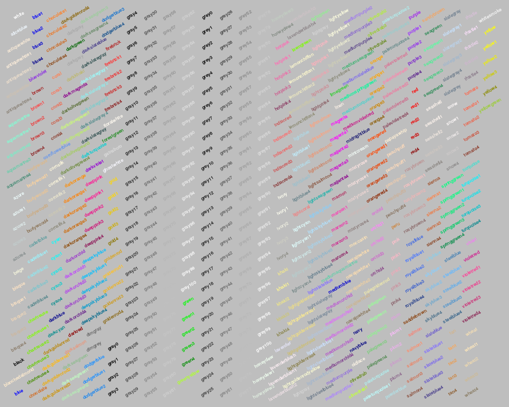
> ## 1) with traditional 'graphics' package:
> showCols1 <- function(bg = "gray", cex = 0.75, srt = 30) {
+ m <- ceiling(sqrt(n <- length(cl <- colors())))
+ length(cl) <- m*m; cm <- matrix(cl, m)
+ ##
+ require("graphics")
+ op <- par(mar=rep(0,4), ann=FALSE, bg = bg); on.exit(par(op))
+ plot(1:m,1:m, type="n", axes=FALSE)
+ text(col(cm), rev(row(cm)), cm, col = cl, cex=cex, srt=srt)
+ }
> showCols1()
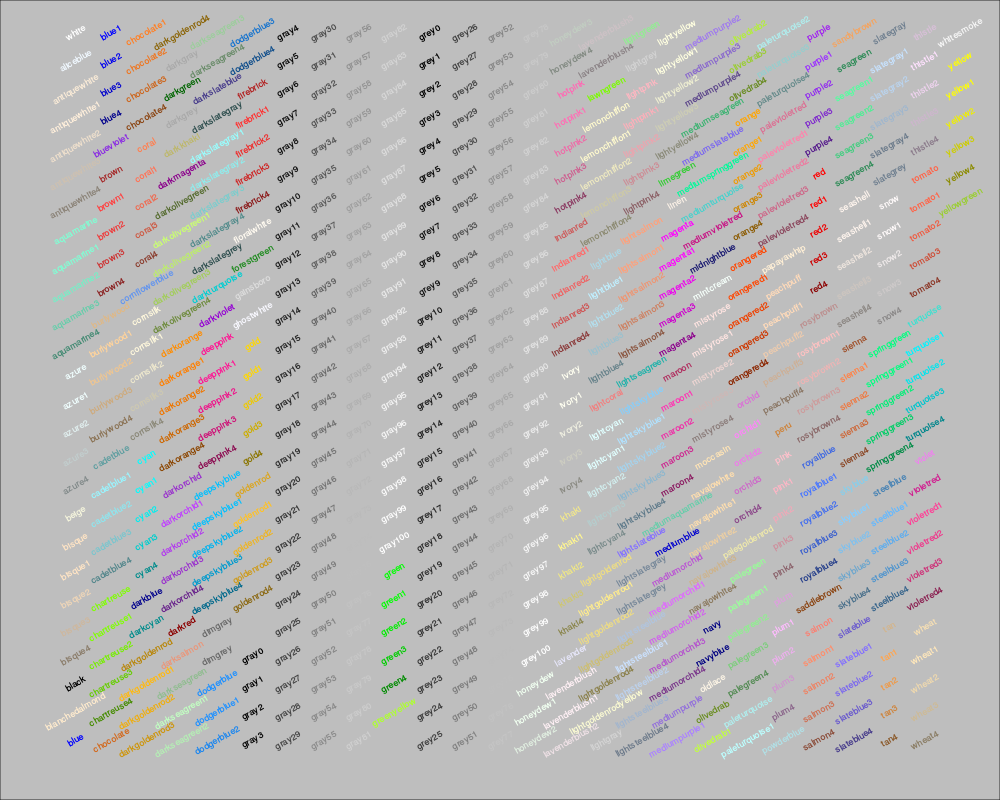
> ## 2) with 'grid' package:
> showCols2 <- function(bg = "grey", cex = 0.75, rot = 30) {
+ m <- ceiling(sqrt(n <- length(cl <- colors())))
+ length(cl) <- m*m; cm <- matrix(cl, m)
+ ##
+ require("grid")
+ grid.newpage(); vp <- viewport(w = .92, h = .92)
+ grid.rect(gp=gpar(fill=bg))
+ grid.text(cm, x = col(cm)/m, y = rev(row(cm))/m, rot = rot,
+ vp=vp, gp=gpar(cex = cex, col = cm))
+ }
> showCols2()
Loading required package: grid
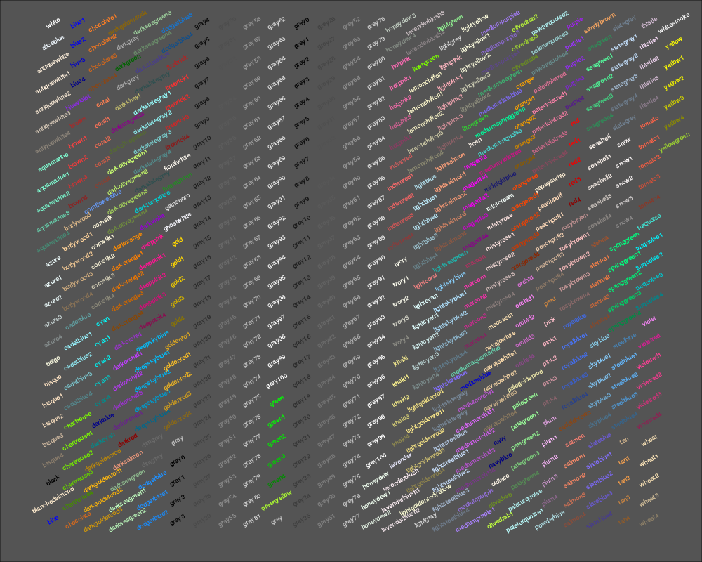
> showCols2(bg = "gray33")
> ###
>
> ##' @title Comparing Colors
> ##' @param col
> ##' @param nrow
> ##' @param ncol
> ##' @param txt.col
> ##' @return the grid layout, invisibly
> ##' @author Marius Hofert, originally
> plotCol <- function(col, nrow=1, ncol=ceiling(length(col) / nrow),
+ txt.col="black") {
+ stopifnot(nrow >= 1, ncol >= 1)
+ if(length(col) > nrow*ncol)
+ warning("some colors will not be shown")
+ require(grid)
+ grid.newpage()
+ gl <- grid.layout(nrow, ncol)
+ pushViewport(viewport(layout=gl))
+ ic <- 1
+ for(i in 1:nrow) {
+ for(j in 1:ncol) {
+ pushViewport(viewport(layout.pos.row=i, layout.pos.col=j))
+ grid.rect(gp= gpar(fill=col[ic]))
+ grid.text(col[ic], gp=gpar(col=txt.col))
+ upViewport()
+ ic <- ic+1
+ }
+ }
+ upViewport()
+ invisible(gl)
+ }
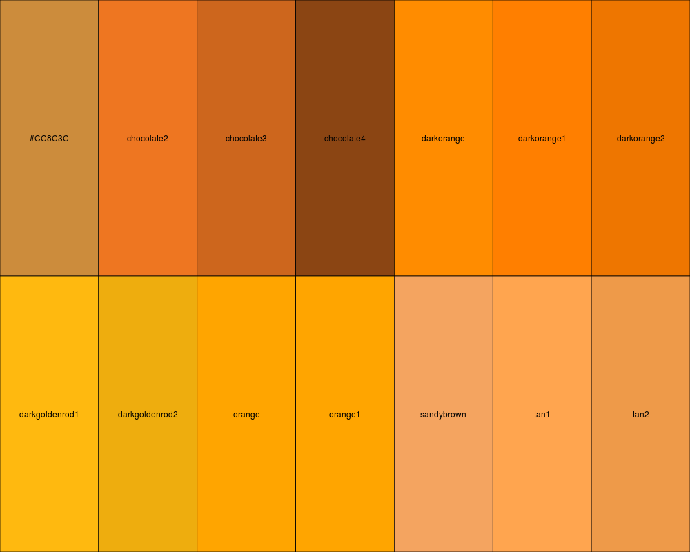
> ## A Chocolate Bar of colors:
> plotCol(c("#CC8C3C", paste0("chocolate", 2:4),
+ paste0("darkorange", c("",1:2)), paste0("darkgoldenrod", 1:2),
+ "orange", "orange1", "sandybrown", "tan1", "tan2"),
+ nrow=2)
> ##' Find close R colors() to a given color {original by Marius Hofert)
> ##' using Euclidean norm in (HSV / RGB / ...) color space
> nearRcolor <- function(rgb, cSpace = c("hsv", "rgb255", "Luv", "Lab"),
+ dist = switch(cSpace, "hsv" = 0.10, "rgb255" = 30,
+ "Luv" = 15, "Lab" = 12))
+ {
+ if(is.character(rgb)) rgb <- col2rgb(rgb)
+ stopifnot(length(rgb <- as.vector(rgb)) == 3)
+ Rcol <- col2rgb(.cc <- colors())
+ uniqC <- !duplicated(t(Rcol)) # gray9 == grey9 (etc)
+ Rcol <- Rcol[, uniqC] ; .cc <- .cc[uniqC]
+ cSpace <- match.arg(cSpace)
+ convRGB2 <- function(Rgb, to)
+ t(convertColor(t(Rgb), from="sRGB", to=to, scale.in=255))
+ ## the transformation, rgb{0..255} --> cSpace :
+ TransF <- switch(cSpace,
+ "rgb255" = identity,
+ "hsv" = rgb2hsv,
+ "Luv" = function(RGB) convRGB2(RGB, "Luv"),
+ "Lab" = function(RGB) convRGB2(RGB, "Lab"))
+ d <- sqrt(colSums((TransF(Rcol) - as.vector(TransF(rgb)))^2))
+ iS <- sort.list(d[near <- d <= dist])# sorted: closest first
+ setNames(.cc[near][iS], format(d[near][iS], digits=3))
+ }
> nearRcolor(col2rgb("tan2"), "rgb")
0.0 21.1 25.8 29.5
"tan2" "tan1" "sandybrown" "sienna1"
> nearRcolor(col2rgb("tan2"), "hsv")
0.0000 0.0410 0.0618 0.0638 0.0667 0.0766
"tan2" "sienna2" "coral2" "tomato2" "tan1" "coral"
0.0778 0.0900 0.0912 0.0918
"sienna1" "sandybrown" "coral1" "tomato"
> nearRcolor(col2rgb("tan2"), "Luv")
0.00 7.42 7.48 12.41 13.69
"tan2" "tan1" "sandybrown" "orange3" "orange2"
> nearRcolor(col2rgb("tan2"), "Lab")
0.00 5.56 8.08 11.31
"tan2" "tan1" "sandybrown" "peru"
> nearRcolor("#334455")
0.0867
"darkslategray"
> ## Now, consider choosing a color by looking in the
> ## neighborhood of one you know :
>
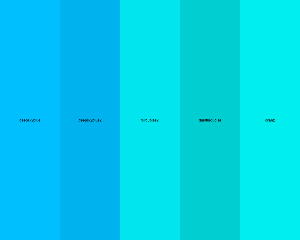
> plotCol(nearRcolor("deepskyblue", "rgb", dist=50))
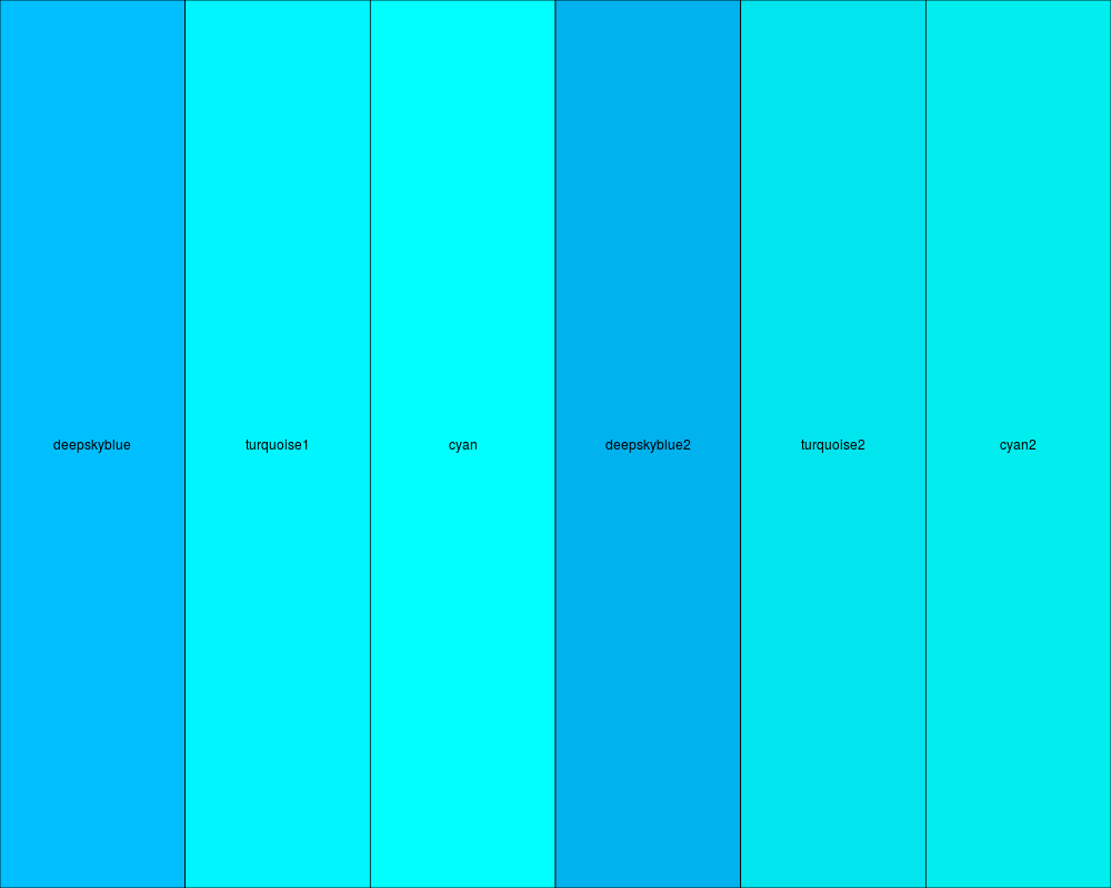
> plotCol(nearRcolor("deepskyblue", dist=.1))
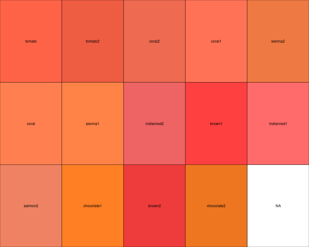
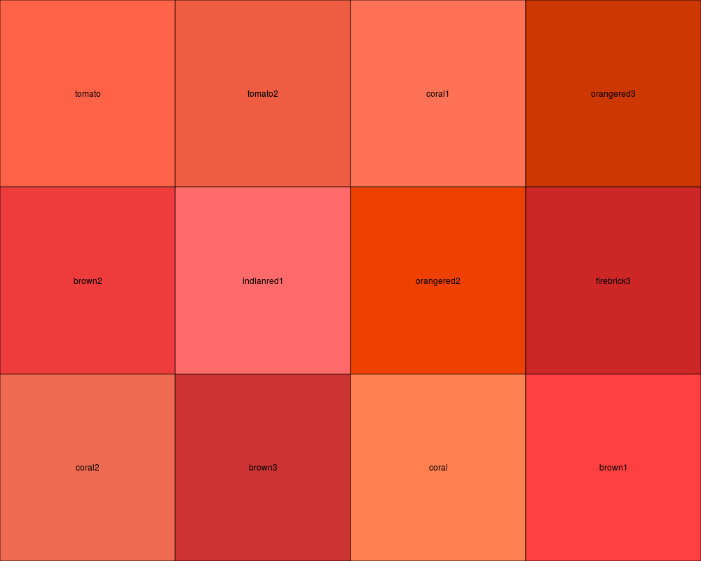
> plotCol(nearRcolor("tomato", "rgb", dist= 50), nrow=3)
> plotCol(nearRcolor("tomato", "hsv", dist=.12), nrow=3)
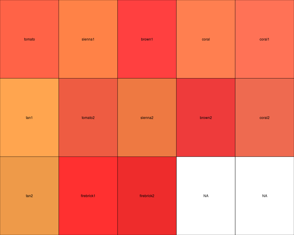
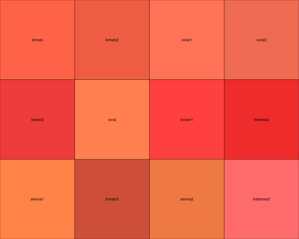
> plotCol(nearRcolor("tomato", "Luv", dist= 25), nrow=3)
> plotCol(nearRcolor("tomato", "Lab", dist= 18), nrow=3)
> ## -----------
>
>
>
>
>
> dev.off()
null device
1
>
|
Created & Maintained by Osamu Ogasawara (osamu.ogasawara@gmail.com) and 