Supported by Dr. Osamu Ogasawara and  . . |
|
Last data update: 2014.03.03 |
Conditioning PlotsDescriptionThis function produces two variants of the conditioning plots discussed in the reference below. Usage
coplot(formula, data, given.values, panel = points, rows, columns,
       show.given = TRUE, col = par("fg"), pch = par("pch"),
       bar.bg = c(num = gray(0.8), fac = gray(0.95)),
       xlab = c(x.name, paste("Given :", a.name)),
       ylab = c(y.name, paste("Given :", b.name)),
       subscripts = FALSE,
       axlabels = function(f) abbreviate(levels(f)),
       number = 6, overlap = 0.5, xlim, ylim, ...)
co.intervals(x, number = 6, overlap = 0.5)
Arguments
DetailsIn the case of a single conditioning variable In the case of multiple A panel function should not attempt to start a new plot, but just plot
within a given coordinate system: thus The rendering of arguments Value
ReferencesChambers, J. M. (1992) Data for models. Chapter 3 of Statistical Models in S eds J. M. Chambers and T. J. Hastie, Wadsworth & Brooks/Cole. Cleveland, W. S. (1993) Visualizing Data. New Jersey: Summit Press. See Also
Examples
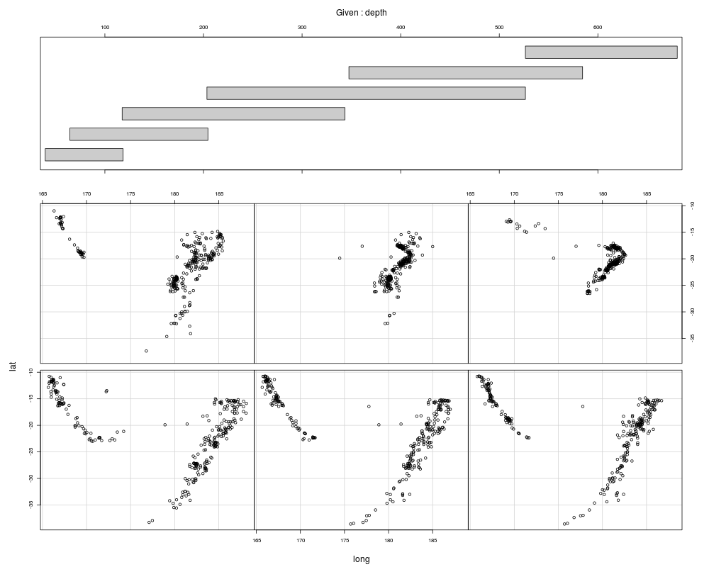
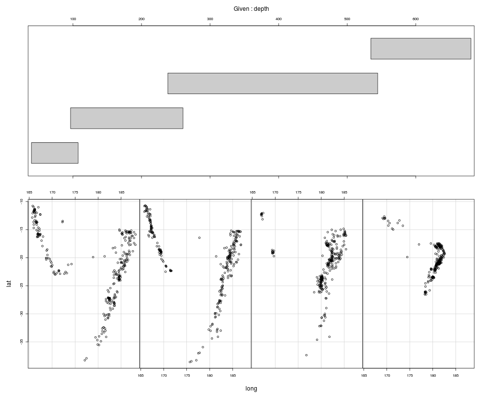
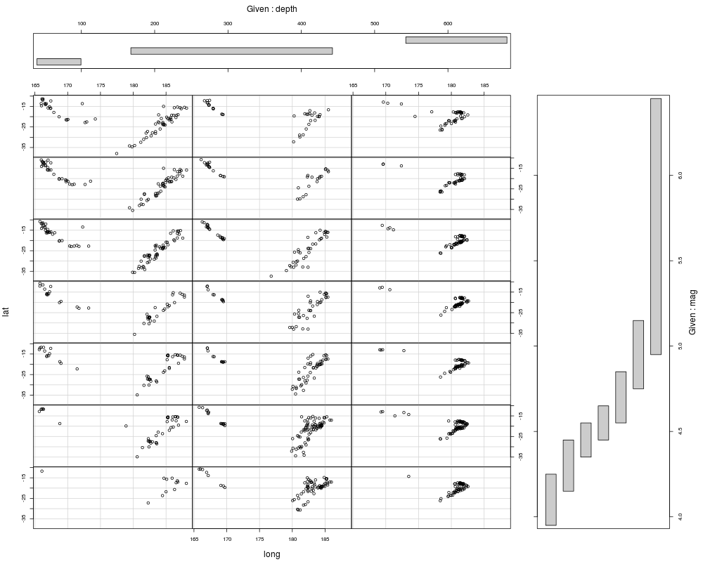
## Tonga Trench Earthquakes
coplot(lat ~ long | depth, data = quakes)
given.depth <- co.intervals(quakes$depth, number = 4, overlap = .1)
coplot(lat ~ long | depth, data = quakes, given.v = given.depth, rows = 1)
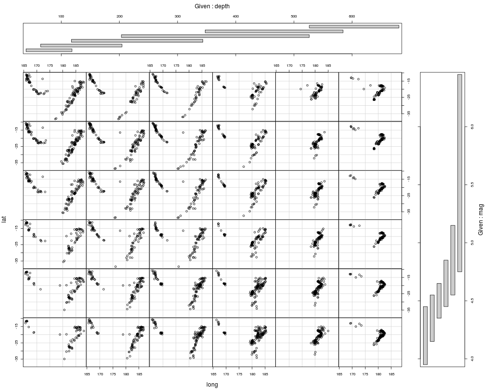
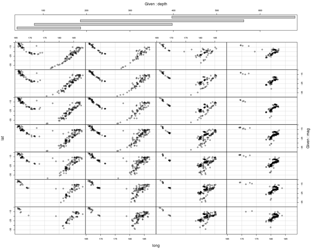
## Conditioning on 2 variables:
ll.dm <- lat ~ long | depth * mag
coplot(ll.dm, data = quakes)
coplot(ll.dm, data = quakes, number = c(4, 7), show.given = c(TRUE, FALSE))
coplot(ll.dm, data = quakes, number = c(3, 7),
overlap = c(-.5, .1)) # negative overlap DROPS values
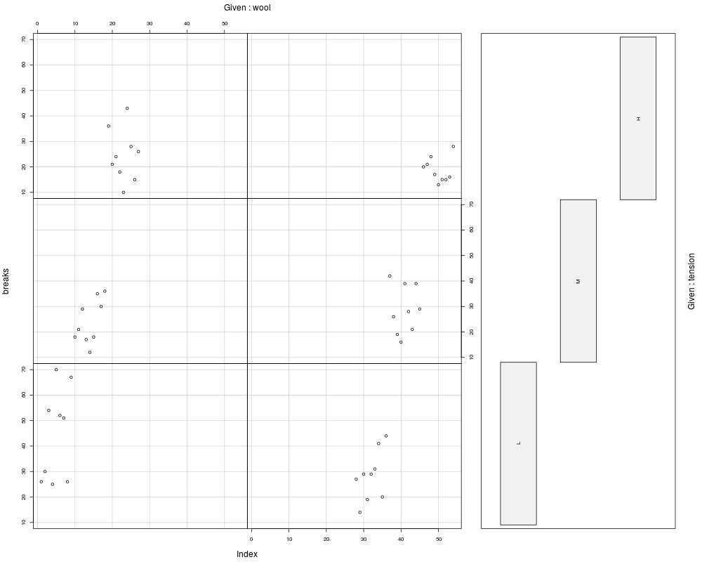
## given two factors
Index <- seq(length = nrow(warpbreaks)) # to get nicer default labels
coplot(breaks ~ Index | wool * tension, data = warpbreaks,
show.given = 0:1)
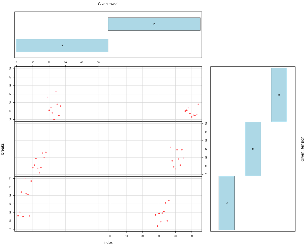
coplot(breaks ~ Index | wool * tension, data = warpbreaks,
col = "red", bg = "pink", pch = 21,
bar.bg = c(fac = "light blue"))
## Example with empty panels:
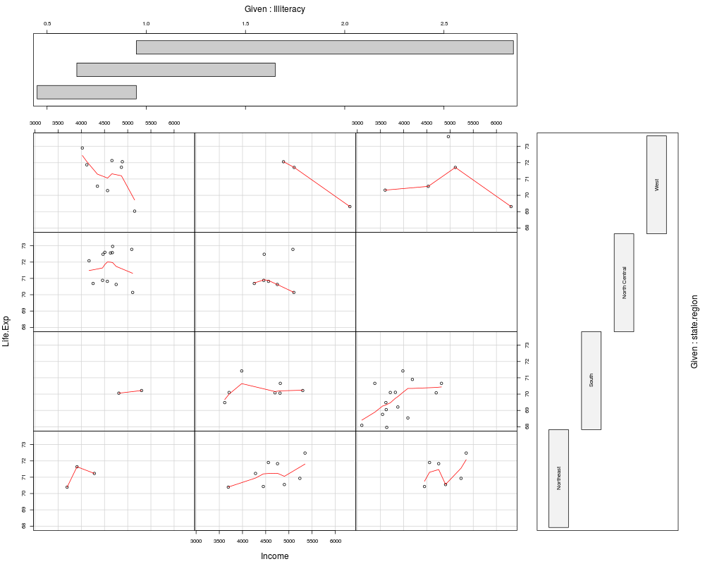
with(data.frame(state.x77), {
coplot(Life.Exp ~ Income | Illiteracy * state.region, number = 3,
panel = function(x, y, ...) panel.smooth(x, y, span = .8, ...))
## y ~ factor -- not really sensible, but 'show off':
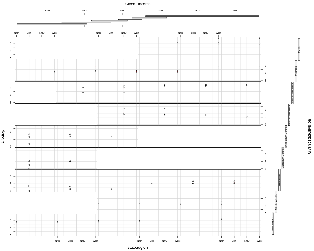
coplot(Life.Exp ~ state.region | Income * state.division,
panel = panel.smooth)
})
Results
R version 3.3.1 (2016-06-21) -- "Bug in Your Hair"
Copyright (C) 2016 The R Foundation for Statistical Computing
Platform: x86_64-pc-linux-gnu (64-bit)

R is free software and comes with ABSOLUTELY NO WARRANTY.
You are welcome to redistribute it under certain conditions.
Type 'license()' or 'licence()' for distribution details.

R is a collaborative project with many contributors.
Type 'contributors()' for more information and
'citation()' on how to cite R or R packages in publications.

Type 'demo()' for some demos, 'help()' for on-line help, or
'help.start()' for an HTML browser interface to help.
Type 'q()' to quit R.

> library(graphics)
> png(filename="/home/ddbj/snapshot/RGM3/R_rel/result/graphics/coplot.Rd_%03d_medium.png", width=480, height=480)
> ### Name: coplot
> ### Title: Conditioning Plots
> ### Aliases: coplot co.intervals
> ### Keywords: hplot aplot
>
> ### ** Examples
>
> ## Tonga Trench Earthquakes
> coplot(lat ~ long | depth, data = quakes)
> given.depth <- co.intervals(quakes$depth, number = 4, overlap = .1)
> coplot(lat ~ long | depth, data = quakes, given.v = given.depth, rows = 1)
>
> ## Conditioning on 2 variables:
> ll.dm <- lat ~ long | depth * mag
> coplot(ll.dm, data = quakes)
> coplot(ll.dm, data = quakes, number = c(4, 7), show.given = c(TRUE, FALSE))
> coplot(ll.dm, data = quakes, number = c(3, 7),
+        overlap = c(-.5, .1)) # negative overlap DROPS values
>
> ## given two factors
> Index <- seq(length = nrow(warpbreaks)) # to get nicer default labels
> coplot(breaks ~ Index | wool * tension, data = warpbreaks,
+        show.given = 0:1)
> coplot(breaks ~ Index | wool * tension, data = warpbreaks,
+        col = "red", bg = "pink", pch = 21,
+        bar.bg = c(fac = "light blue"))
>
> ## Example with empty panels:
> with(data.frame(state.x77), {
+ coplot(Life.Exp ~ Income | Illiteracy * state.region, number = 3,
+        panel = function(x, y, ...) panel.smooth(x, y, span = .8, ...))
+ ## y ~ factor -- not really sensible, but 'show off':
+ coplot(Life.Exp ~ state.region | Income * state.division,
+        panel = panel.smooth)
+ })
>
>
>
>
>
> dev.off()
null device
          1
>
|