R Graphical Manual

Browse All

Last data update: 2014.03.03

R: Generic X-Y Plotting

plot	R Documentation

Generic X-Y Plotting

Description

Generic function for plotting of R objects. For more details about the graphical parameter arguments, see par.

For simple scatter plots, plot.default will be used. However, there are plot methods for many R objects, including functions, data.frames, density objects, etc. Use methods(plot) and the documentation for these.

Usage

plot(x, y, ...)

Arguments

x

the coordinates of points in the plot. Alternatively, a single plotting structure, function or any R object with a plot method can be provided.

y

the y coordinates of points in the plot, optional if x is an appropriate structure.

...

Arguments to be passed to methods, such as graphical parameters (see par). Many methods will accept the following arguments:

type

what type of plot should be drawn. Possible types are

"p" for points,
"l" for lines,
"b" for both,
"c" for the lines part alone of "b",
"o" for both ‘overplotted’,
"h" for ‘histogram’ like (or ‘high-density’) vertical lines,
"s" for stair steps,
"S" for other steps, see ‘Details’ below,
"n" for no plotting.

All other types give a warning or an error; using, e.g., type = "punkte" being equivalent to type = "p" for S compatibility. Note that some methods, e.g. plot.factor, do not accept this.

main

an overall title for the plot: see title.

sub

a sub title for the plot: see title.

xlab

a title for the x axis: see title.

ylab

a title for the y axis: see title.

asp

the y/x aspect ratio, see plot.window.

Details

The two step types differ in their x-y preference: Going from (x1,y1) to (x2,y2) with x1 < x2, type = "s" moves first horizontal, then vertical, whereas type = "S" moves the other way around.

Examples

require(stats) # for lowess, rpois, rnorm
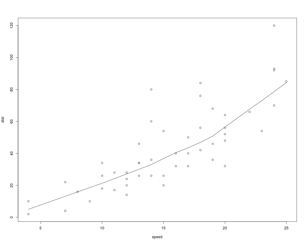
plot(cars)
lines(lowess(cars))

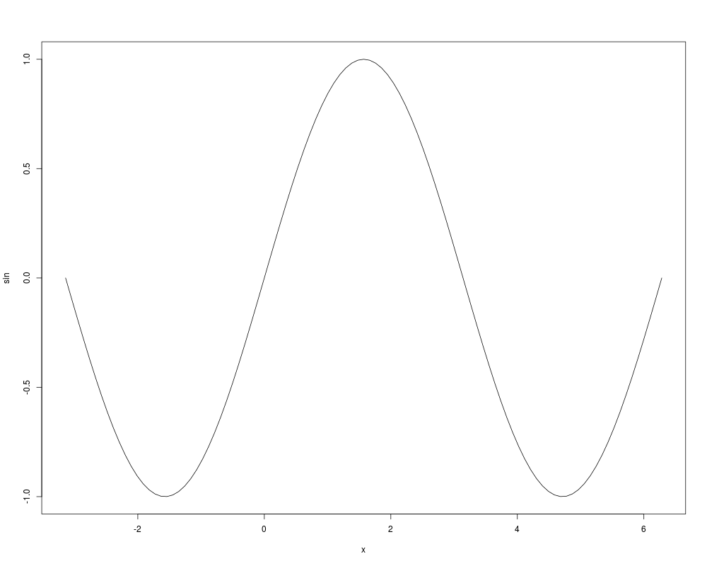
plot(sin, -pi, 2*pi) # see ?plot.function

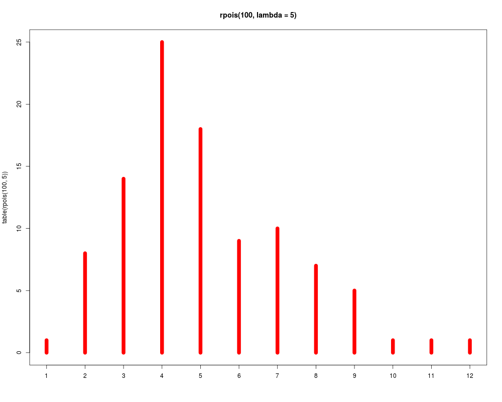
## Discrete Distribution Plot:
plot(table(rpois(100, 5)), type = "h", col = "red", lwd = 10,
     main = "rpois(100, lambda = 5)")

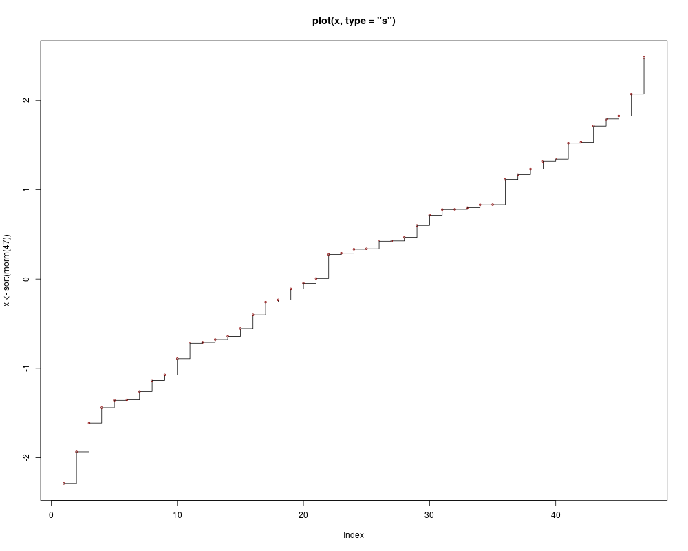
## Simple quantiles/ECDF, see ecdf() {library(stats)} for a better one:
plot(x <- sort(rnorm(47)), type = "s", main = "plot(x, type = "s")")
points(x, cex = .5, col = "dark red")

Results


R version 3.3.1 (2016-06-21) -- "Bug in Your Hair"
Copyright (C) 2016 The R Foundation for Statistical Computing
Platform: x86_64-pc-linux-gnu (64-bit)

R is free software and comes with ABSOLUTELY NO WARRANTY.
You are welcome to redistribute it under certain conditions.
Type 'license()' or 'licence()' for distribution details.

R is a collaborative project with many contributors.
Type 'contributors()' for more information and
'citation()' on how to cite R or R packages in publications.

Type 'demo()' for some demos, 'help()' for on-line help, or
'help.start()' for an HTML browser interface to help.
Type 'q()' to quit R.

> library(graphics)
> png(filename="/home/ddbj/snapshot/RGM3/R_rel/result/graphics/plot.Rd_%03d_medium.png", width=480, height=480)
> ### Name: plot
> ### Title: Generic X-Y Plotting
> ### Aliases: plot
> ### Keywords: hplot
> 
> ### ** Examples
> 
> require(stats) # for lowess, rpois, rnorm
> plot(cars)
> lines(lowess(cars))
> 
> plot(sin, -pi, 2*pi) # see ?plot.function
> 
> ## Discrete Distribution Plot:
> plot(table(rpois(100, 5)), type = "h", col = "red", lwd = 10,
+      main = "rpois(100, lambda = 5)")
> 
> ## Simple quantiles/ECDF, see ecdf() {library(stats)} for a better one:
> plot(x <- sort(rnorm(47)), type = "s", main = "plot(x, type = "s")")
> points(x, cex = .5, col = "dark red")
> 
> 
> 
> 
> 
> dev.off()
null device 
          1 
>