R Graphical Manual

Browse All

Last data update: 2014.03.03

R: Calculation Of Predicition Profiles

getPredictionProfile,BioVector-method

R Documentation

Calculation Of Predicition Profiles

Description

compute prediction profiles for a given set of biological sequences from a model trained with /codekbsvm

Usage

## S4 method for signature 'BioVector'
getPredictionProfile(object, kernel, featureWeights, b,
  svmIndex = 1, sel = NULL, weightLimit = .Machine$double.eps)

## S4 method for signature 'XStringSet'
getPredictionProfile(object, kernel, featureWeights, b,
  svmIndex = 1, sel = NULL, weightLimit = .Machine$double.eps)

## S4 method for signature 'XString'
getPredictionProfile(object, kernel, featureWeights, b,
  svmIndex = 1, sel = NULL, weightLimit = .Machine$double.eps)

Arguments

`object`	a single biological sequence in the form of an `DNAString`, `RNAString` or `AAString` or multiple biological sequences as `DNAStringSet`, `RNAStringSet`, `AAStringSet` (or as `BioVector`).
`kernel`	a sequence kernel object of class `SequenceKernel`.
`featureWeights`	a feature weights matrix retrieved from a KeBABS model with the accessor `featureWeights`.
`b`	model intercept from a KeBABS model.
`svmIndex`	integer value selecting one of the pairwise SVMs in case of pairwise multiclass classification. Default=1
`sel`	subset of indices into `x` as integer vector. When this parameter is present the prediction profiles are computed for the specified subset of samples only. Default=`integer(0)`
`weightLimit`	the feature weight limit is a single numeric value and allows pruning of feature weights. All feature weights with an absolute value below this limit are set to 0 and are not considered for the prediction profile computation. This parameter is only relevant when feature weights are calculated in KeBABS during training. Default=.Machine$double.eps

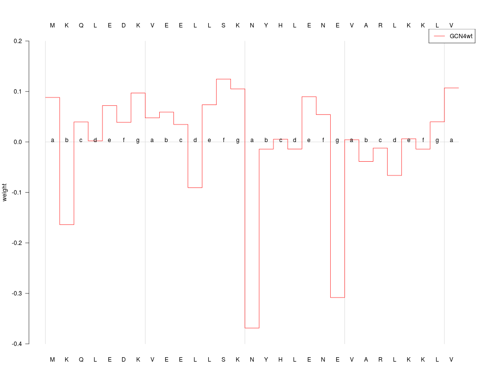
Details

With this method prediction profiles can be generated explicitely for a given set of sequences with a given model represented through its feature weights and the model intercept b. A single prediction profile shows for each position of the sequence the contribution of the patterns at this position to the decision value. The prediciion profile also includes the kernel object used for the generation of the profile and the seqence data.

A single profile or a pair can be plotted with method plot showing the relevance of sequence positions for the prediction. Please consider that patterns occuring at neighboring sequence positions are not statistically independent which means that the relevance of a specific position is not only determined by the patterns at this position but is also influenced by the neighborhood around this position. Prediction profiles can also be generated implicitely during predction for the predicted samples (see parameter predProfiles in predict).

Value

getPredictionProfile: upon successful completion, the function returns a set of prediction profiles for the sequences as class PredictionProfile.

Author(s)

Johannes Palme <kebabs@bioinf.jku.at>

References

http://www.bioinf.jku.at/software/kebabs

(Mahrenholz, 2011) – C.C. Mahrenholz, I.G. Abfalter, U. Bodenhofer, R. Volkmer, and S. Hochreiter. Complex networks govern coiled coil oligomerization - predicting and profiling by means of a machine learning approach.

(Bodenhofer, 2009) – U. Bodenhofer, K. Schwarzbauer, S. Ionescu, and S. Hochreiter. Modeling Position Specificity in Sequence Kernels by Fuzzy Equivalence Relations.

J. Palme, S. Hochreiter, and U. Bodenhofer (2015) KeBABS: an R package for kernel-based analysis of biological sequences. Bioinformatics, 31(15):2574-2576, 2015. DOI: 10.1093/bioinformatics/btv176.

Examples

## set random generator seed to make the results of this example
## reproducable
set.seed(123)

## load coiled coil data
data(CCoil)
gappya <- gappyPairKernel(k=1,m=11, annSpec=TRUE)
model <- kbsvm(x=ccseq, y=as.numeric(yCC), kernel=gappya,
               pkg="e1071", svm="C-svc", cost=15)

## show feature weights
featureWeights(model)[,1:5]

## define two new sequences to be predicted
GCN4 <- AAStringSet(c("MKQLEDKVEELLSKNYHLENEVARLKKLV",
                      "MKQLEDKVEELLSKYYHTENEVARLKKLV"))
names(GCN4) <- c("GCN4wt", "GCN_N16Y,L19T")
## assign annotation metadata
annCharset <- annotationCharset(ccseq)
annot <- c("abcdefgabcdefgabcdefgabcdefga",
           "abcdefgabcdefgabcdefgabcdefga")
annotationMetadata(GCN4, annCharset=annCharset) <- annot

## compute prediction profiles
predProf <- getPredictionProfile(GCN4, gappya,
           featureWeights(model), modelOffset(model))

## show prediction profiles
predProf

## plot prediction profile of first aa sequence
plot(predProf, sel=1, ylim=c(-0.4, 0.2), heptads=TRUE, annotate=TRUE)

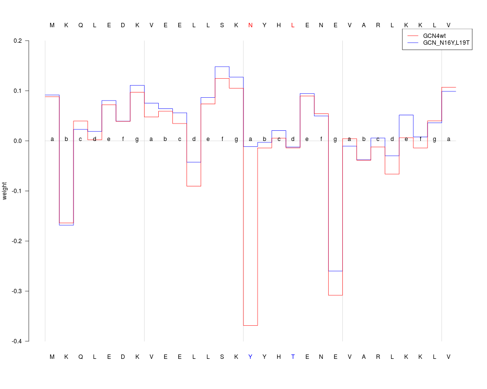
## plot prediction profile of both aa sequences
plot(predProf, sel=c(1,2), ylim=c(-0.4, 0.2), heptads=TRUE, annotate=TRUE)

## prediction profiles can also be generated during prediction
## when setting the parameter predProf to TRUE
## plotting longer sequences to pdf is shown in the examples for the
## plot function

Results


R version 3.3.1 (2016-06-21) -- "Bug in Your Hair"
Copyright (C) 2016 The R Foundation for Statistical Computing
Platform: x86_64-pc-linux-gnu (64-bit)

R is free software and comes with ABSOLUTELY NO WARRANTY.
You are welcome to redistribute it under certain conditions.
Type 'license()' or 'licence()' for distribution details.

R is a collaborative project with many contributors.
Type 'contributors()' for more information and
'citation()' on how to cite R or R packages in publications.

Type 'demo()' for some demos, 'help()' for on-line help, or
'help.start()' for an HTML browser interface to help.
Type 'q()' to quit R.

> library(kebabs)
Loading required package: Biostrings
Loading required package: BiocGenerics
Loading required package: parallel

Attaching package: 'BiocGenerics'

The following objects are masked from 'package:parallel':

    clusterApply, clusterApplyLB, clusterCall, clusterEvalQ,
    clusterExport, clusterMap, parApply, parCapply, parLapply,
    parLapplyLB, parRapply, parSapply, parSapplyLB

The following objects are masked from 'package:stats':

    IQR, mad, xtabs

The following objects are masked from 'package:base':

    Filter, Find, Map, Position, Reduce, anyDuplicated, append,
    as.data.frame, cbind, colnames, do.call, duplicated, eval, evalq,
    get, grep, grepl, intersect, is.unsorted, lapply, lengths, mapply,
    match, mget, order, paste, pmax, pmax.int, pmin, pmin.int, rank,
    rbind, rownames, sapply, setdiff, sort, table, tapply, union,
    unique, unsplit

Loading required package: S4Vectors
Loading required package: stats4

Attaching package: 'S4Vectors'

The following objects are masked from 'package:base':

    colMeans, colSums, expand.grid, rowMeans, rowSums

Loading required package: IRanges
Loading required package: XVector
Loading required package: kernlab

Attaching package: 'kernlab'

The following object is masked from 'package:Biostrings':

    type

> png(filename="/home/ddbj/snapshot/RGM3/R_BC/result/kebabs/getPredictionProfile-methods.Rd_%03d_medium.png", width=480, height=480)
> ### Name: getPredictionProfile,BioVector-method
> ### Title: Calculation Of Predicition Profiles
> ### Aliases: getPredictionProfile getPredictionProfile,BioVector-method
> ###   getPredictionProfile,XString-method
> ###   getPredictionProfile,XStringSet-method
> ### Keywords: feature methods prediction profile weights
> 
> ### ** Examples
> 
> ## set random generator seed to make the results of this example
> ## reproducable
> set.seed(123)
> 
> ## load coiled coil data
> data(CCoil)
> gappya <- gappyPairKernel(k=1,m=11, annSpec=TRUE)
> model <- kbsvm(x=ccseq, y=as.numeric(yCC), kernel=gappya,
+                pkg="e1071", svm="C-svc", cost=15)
> 
> ## show feature weights
> featureWeights(model)[,1:5]
    A......Aa......a                 AAab   A.......Aa.......b 
          0.11453726           0.11933186           0.04043841 
              A.Aa.c A........Aa........c 
         -0.08263644           0.05626802 
> 
> ## define two new sequences to be predicted
> GCN4 <- AAStringSet(c("MKQLEDKVEELLSKNYHLENEVARLKKLV",
+                       "MKQLEDKVEELLSKYYHTENEVARLKKLV"))
> names(GCN4) <- c("GCN4wt", "GCN_N16Y,L19T")
> ## assign annotation metadata
> annCharset <- annotationCharset(ccseq)
> annot <- c("abcdefgabcdefgabcdefgabcdefga",
+            "abcdefgabcdefgabcdefgabcdefga")
> annotationMetadata(GCN4, annCharset=annCharset) <- annot
> 
> ## compute prediction profiles
> predProf <- getPredictionProfile(GCN4, gappya,
+            featureWeights(model), modelOffset(model))
> 
> ## show prediction profiles
> predProf
An object of class  "PredictionProfile" 

Sequences:

  A AAStringSet instance of length 2
    width seq                                               names               
[1]    29 MKQLEDKVEELLSKNYHLENEVARLKKLV                     GCN4wt
[2]    29 MKQLEDKVEELLSKYYHTENEVARLKKLV                     GCN_N16Y,L19T

gappy pair kernel: k=1, m=11, annSpec=TRUE

Baselines:  0.02365245 0.02365245 

Profiles:
                     Pos 1        Pos 2            Pos 28       Pos 29 
       GCN4wt  0.111889252 -0.140135744  ...  0.063537667  0.130766121
GCN_N16Y,L19T  0.115429679 -0.144569953  ...  0.059671695  0.122502550

> 
> ## plot prediction profile of first aa sequence
> plot(predProf, sel=1, ylim=c(-0.4, 0.2), heptads=TRUE, annotate=TRUE)
> 
> ## plot prediction profile of both aa sequences
> plot(predProf, sel=c(1,2), ylim=c(-0.4, 0.2), heptads=TRUE, annotate=TRUE)
> 
> ## prediction profiles can also be generated during prediction
> ## when setting the parameter predProf to TRUE
> ## plotting longer sequences to pdf is shown in the examples for the
> ## plot function
> 
> 
> 
> 
> 
> dev.off()
null device 
          1 
>