Supported by Dr. Osamu Ogasawara and  . . |
|
Last data update: 2014.03.03 |
Plot Prediction Profiles, Cross Validation Result, Grid Search Performance Parameters and Receiver Operating CharacteristicsDescriptionFunctions for visualizing prediction profiles, cross validation result, grid search performance parameters and receiver operating characteristics Usage
## S4 method for signature 'PredictionProfile,missing'
plot(x, sel = NULL, col = c("red",
  "blue"), standardize = TRUE, shades = NULL, legend = "default",
  legendPos = "topright", ylim = NULL, xlab = "", ylab = "weight",
  lwd.profile = 1, lwd.axis = 1, las = 1, heptads = FALSE,
  annotate = FALSE, markOffset = TRUE, windowSize = 1, ...)

## S4 method for signature 'CrossValidationResult,missing'
plot(x, col = "springgreen")

## S4 method for signature 'ModelSelectionResult,missing'
plot(x, sel = c("ACC", "BACC", "MCC",
  "AUC"))

## S4 method for signature 'ROCData,missing'
plot(x, lwd = 2, aucDigits = 3, cex = 0.8,
  side = 1, line = -3, adj = 0.9, ...)
Arguments
DetailsPlotting of Prediction Profiles The baseline for the step function of a single sample represents the offset b of the model distributed equally to all sequence positions according to the following reformulation of the discriminant function f(x) = b + sum(si(x)) = sum(si(x) -(-b/L)) for i = 1, ... L For standardized plots (see parameter When plotting to a pdf it is recommended to use a height to width ratio
of around 1:(max sequence length/25), e.g. for a maximum sequence length
of 500 bases or amino acids select height=10 and width=200 when opening the
pdf document for plotting. Plotting of CrossValidation Result Plotting of Grid Performance Values Plotting of Receiver Operating Characteristics (ROC) Valuesee details above Author(s)Johannes Palme <kebabs@bioinf.jku.at> Referenceshttp://www.bioinf.jku.at/software/kebabs See Also
Examples
## set seed for random generator, included here only to make results
## reproducable for this example
set.seed(456)
## load transcription factor binding site data
data(TFBS)
enhancerFB
## select 70% of the samples for training and the rest for test
train <- sample(1:length(enhancerFB), length(enhancerFB) * 0.7)
test <- c(1:length(enhancerFB))[-train]
## create the kernel object for gappy pair kernel with normalization
gappy <- gappyPairKernel(k=1, m=3)
## show details of kernel object
gappy
## run training with explicit representation
model <- kbsvm(x=enhancerFB[train], y=yFB[train], kernel=gappy,
pkg="LiblineaR", svm="C-svc", cost=80, explicit="yes",
featureWeights="yes")
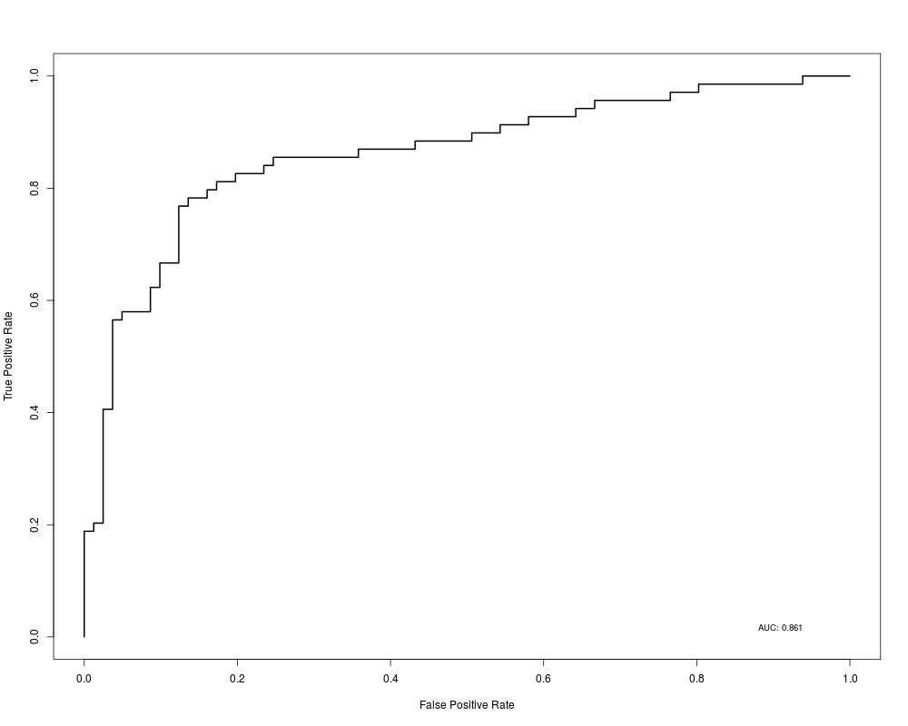
## compute and plot ROC for test sequences
preddec <- predict(model, enhancerFB[test], predictionType="decision")
rocdata <- computeROCandAUC(preddec, yFB[test], allLabels=unique(yFB))
plot(rocdata)
## generate prediction profile for the first three test sequences
predProf <- getPredictionProfile(enhancerFB, gappy, featureWeights(model),
modelOffset(model), sel=test[1:3])
## show prediction profiles
predProf
## plot prediction profile to pdf
## As sequences are usually very long select a ratio of height to width
## for the pdf which takes care of the maximum sequence length which is
## plotted. Only single or pairs of prediction profiles can be plotted.
## Plot profile for window size 1 (default) and 50. Load package Biobase
## for openPDF
## Not run:
library(Biobase)
pdf(file="PredictionProfile1_w1.pdf", height=10, width=200)
plot(predProf, sel=c(1,3))
dev.off()
openPDF("PredictionProfile1_w1.pdf")
pdf(file="PredictionProfile1_w50.pdf", height=10, width=200)
plot(predProf, sel=c(1,3), windowSize=50)
dev.off()
openPDF("PredictionProfile1_w50.pdf")
pdf(file="PredictionProfile2_w1.pdf", height=10, width=200)
plot(predProf, sel=c(2,3))
dev.off()
openPDF("PredictionProfile2_w1.pdf")
pdf(file="PredictionProfile2_w50.pdf", height=10, width=200)
plot(predProf, sel=c(2,3), windowSize=50)
dev.off()
openPDF("PredictionProfile2_w50.pdf")
## End(Not run)
Results
R version 3.3.1 (2016-06-21) -- "Bug in Your Hair"
Copyright (C) 2016 The R Foundation for Statistical Computing
Platform: x86_64-pc-linux-gnu (64-bit)

R is free software and comes with ABSOLUTELY NO WARRANTY.
You are welcome to redistribute it under certain conditions.
Type 'license()' or 'licence()' for distribution details.

R is a collaborative project with many contributors.
Type 'contributors()' for more information and
'citation()' on how to cite R or R packages in publications.

Type 'demo()' for some demos, 'help()' for on-line help, or
'help.start()' for an HTML browser interface to help.
Type 'q()' to quit R.

> library(kebabs)
Loading required package: Biostrings
Loading required package: BiocGenerics
Loading required package: parallel

Attaching package: 'BiocGenerics'

The following objects are masked from 'package:parallel':

    clusterApply, clusterApplyLB, clusterCall, clusterEvalQ,
    clusterExport, clusterMap, parApply, parCapply, parLapply,
    parLapplyLB, parRapply, parSapply, parSapplyLB

The following objects are masked from 'package:stats':

    IQR, mad, xtabs

The following objects are masked from 'package:base':

    Filter, Find, Map, Position, Reduce, anyDuplicated, append,
    as.data.frame, cbind, colnames, do.call, duplicated, eval, evalq,
    get, grep, grepl, intersect, is.unsorted, lapply, lengths, mapply,
    match, mget, order, paste, pmax, pmax.int, pmin, pmin.int, rank,
    rbind, rownames, sapply, setdiff, sort, table, tapply, union,
    unique, unsplit

Loading required package: S4Vectors
Loading required package: stats4

Attaching package: 'S4Vectors'

The following objects are masked from 'package:base':

    colMeans, colSums, expand.grid, rowMeans, rowSums

Loading required package: IRanges
Loading required package: XVector
Loading required package: kernlab

Attaching package: 'kernlab'

The following object is masked from 'package:Biostrings':

    type

> png(filename="/home/ddbj/snapshot/RGM3/R_BC/result/kebabs/plot-methods.Rd_%03d_medium.png", width=480, height=480)
> ### Name: plot,PredictionProfile,missing-method
> ### Title: Plot Prediction Profiles, Cross Validation Result, Grid Search
> ###   Performance Parameters and Receiver Operating Characteristics
> ### Aliases: plot plot,CrossValidationResult,missing-method
> ###   plot,CrossValidationResult-method
> ###   plot,ModelSelectionResult,missing-method
> ###   plot,ModelSelectionResult-method
> ###   plot,PredictionProfile,missing-method plot,PredictionProfile-method
> ###   plot,ROCData,missing-method plot,ROCData-method
> ### Keywords: methods plot prediction profile
>
> ### ** Examples
>
> ## set seed for random generator, included here only to make results
> ## reproducable for this example
> set.seed(456)
> ## load transcription factor binding site data
> data(TFBS)
> enhancerFB
  A DNAStringSet instance of length 500
      width seq                                             names
  [1]   827 ACTAAACAACATCAATCAATAC...TTCTCTAGGCAAAATCCTGACA chr19.21240050.21...
  [2]   678 GAATATAGACCCTTGGTGGTGG...GGAGGAAGTTATATTAATTTAT chr2.144463827.14...
  [3]   878 CACCCACATGGTGGCTCTCAAC...TCTGCTCCCCACTGTATCACTC chr7.38525408.385...
  [4]   927 TGCCGTAGTGTGCCAGCTTTTC...TTCTCTGATTCTCCTGGATCAA chr4.90747075.907...
  [5]   953 CTTCATATACCTATTAATTCAG...AATAACCTAATTTAAAAAGGGG chr4.9148679.9149631
  ...   ... ...
[496]   478 ACGAGAATGAGGGAAAGCACTG...TTGCAGTCTGCCTTCCGAGTGA chr8.45499713.455...
[497]  1552 AGGGGACTGGAAGAAAGGAACC...AGATCTCTCTTCTAAGCGAGCA chr8.94657200.946...
[498]   503 GATGAACGTAAAATGCAAGCTG...GAACCTAATGACTCCCTTCTGA chr17.73900306.73...
[499]  1577 ACCCCTCTGAGACCAAGAGGTG...GGCAAGTAGGTCTGTATTCCTG chr9.90587075.905...
[500]   778 CACTGTCATAACTTGCTTTCTA...GGCTTGTAGAGTAGCTGCTCTC chr17.48680137.48...
> ## select 70% of the samples for training and the rest for test
> train <- sample(1:length(enhancerFB), length(enhancerFB) * 0.7)
> test <- c(1:length(enhancerFB))[-train]
> ## create the kernel object for gappy pair kernel with normalization
> gappy <- gappyPairKernel(k=1, m=3)
> ## show details of kernel object
> gappy
gappy pair kernel: k=1, m=3
>
> ## run training with explicit representation
> model <- kbsvm(x=enhancerFB[train], y=yFB[train], kernel=gappy,
+                pkg="LiblineaR", svm="C-svc", cost=80, explicit="yes",
+                featureWeights="yes")
>
> ## compute and plot ROC for test sequences
> preddec <- predict(model, enhancerFB[test], predictionType="decision")
> rocdata <- computeROCandAUC(preddec, yFB[test], allLabels=unique(yFB))
> plot(rocdata)
>
> ## generate prediction profile for the first three test sequences
> predProf <- getPredictionProfile(enhancerFB, gappy, featureWeights(model),
+                                  modelOffset(model), sel=test[1:3])
>
> ## show prediction profiles
> predProf
An object of class  "PredictionProfile"

Sequences:

  A DNAStringSet instance of length 3
    width seq                                               names
[1]   878 CACCCACATGGTGGCTCTCAACC...CTCTGCTCCCCACTGTATCACTC chr7.38525408.385...
[2]   927 TGCCGTAGTGTGCCAGCTTTTCG...TTTCTCTGATTCTCCTGGATCAA chr4.90747075.907...
[3]   803 TACCTTAAGGAAATACAGACAAG...GCTCTAGCAGGGCTTTGTGAAGA chr5.113189184.11...

gappy pair kernel: k=1, m=3

Baselines:  0.01223163 0.01158508 0.01337406

Profiles:
                           Pos 1       Pos 2          Pos 926     Pos 927
chr7.38525408.385...  0.02608203 -0.00241429  ...  0.00000000  0.00000000
chr4.90747075.907... -0.00542039  0.03740036  ...  0.03051739  0.01590914
chr5.113189184.11... -0.01496562 -0.04417322  ...  0.00000000  0.00000000

>
> ## plot prediction profile to pdf
> ## As sequences are usually very long select a ratio of height to width
> ## for the pdf which takes care of the maximum sequence length which is
> ## plotted. Only single or pairs of prediction profiles can be plotted.
> ## Plot profile for window size 1 (default) and 50. Load package Biobase
> ## for openPDF
> ## Not run:
> ##D library(Biobase)
> ##D pdf(file="PredictionProfile1_w1.pdf", height=10, width=200)
> ##D plot(predProf, sel=c(1,3))
> ##D dev.off()
> ##D openPDF("PredictionProfile1_w1.pdf")
> ##D pdf(file="PredictionProfile1_w50.pdf", height=10, width=200)
> ##D plot(predProf, sel=c(1,3), windowSize=50)
> ##D dev.off()
> ##D openPDF("PredictionProfile1_w50.pdf")
> ##D pdf(file="PredictionProfile2_w1.pdf", height=10, width=200)
> ##D plot(predProf, sel=c(2,3))
> ##D dev.off()
> ##D openPDF("PredictionProfile2_w1.pdf")
> ##D pdf(file="PredictionProfile2_w50.pdf", height=10, width=200)
> ##D plot(predProf, sel=c(2,3), windowSize=50)
> ##D dev.off()
> ##D openPDF("PredictionProfile2_w50.pdf")
> ## End(Not run)
>
>
>
>
>
> dev.off()
null device
          1
>
|