R Graphical Manual

Browse All

Last data update: 2014.03.03

R: Plot a 'Biplot' of a SelectVar class object

Biplot

R Documentation

Plot a `Biplot` of a SelectVar class object

Description

Plot a Biplot of a SelectVar class object

Usage

## S4 method for signature 'SelectVar'
Biplot(x,xlab=NULL, ylab=NULL, mainP=NULL,
xlimi=NULL, ylimi=NULL, labelObs=TRUE,labelVars= TRUE,
colVar= "black",colObs="black",
 pchPoints=15,Type=c("RMP","CMP","SQRT","HJ"),
 Groups=FALSE,NGroups=2 ,...)

Arguments

`x`	DiStatis class object.
`xlab`	character for the x-label title for plot
`ylab`	character for the x-label title for plot
`mainP`	the main Biplot
`xlimi`	(vector) Bounds to x-axis
`ylimi`	(vector) Bounds to y-axis
`labelObs`	Logical. indicates whether the labels of observations are prints. Default is TRUE
`labelVars`	Logical. indicates whether the labels of variables are prints. Default is TRUE
`colVar`	character col for colours of the variables in the plot. Default is black.
`colObs`	character col for colours of the observations in the plot. Default is black.
`pchPoints`	Either an integer specifying a symbol or a single character to be used as the default in plotting points.
`Type`	type of Biplot. Options are CMP RMP SQRT or HJ.
`Groups`	Logical. If is TRUE, the variables are grouped. See `GroupProj`
`NGroups`	Only if the Groups are TRUE. Indicate the number the groups of variables.
`...`	additional parameters for plot

Value

plotted Biplot/s of the component/s of the given SelectVar object.

Author(s)

M L Zingaretti, J A Demey-Zambrano, J L Vicente Villardon, J R Demey

Examples

{
data(NCI60Selec)
Z1<-DiStatis(NCI60Selec)
M1<-SelectVar(Z1,Crit="R2-Adj")
Colores1<-c(rep("Breast",5),rep("CNS",6),rep("Colon",7),
rep("Leukemia",6),rep("Melanoma",10),rep("Lung",9),
rep("Ovarian",7),rep("Prostate",2),rep("Renal",8))
Colores2<-c(rep(colors()[657],5),rep(colors()[637],6),
rep(colors()[537],7),rep(colors()[552],6),rep(colors()[57],10)
,rep(colors()[300],9),rep(colors()[461],7),rep(colors()[450],2)
,rep(colors()[432],8))
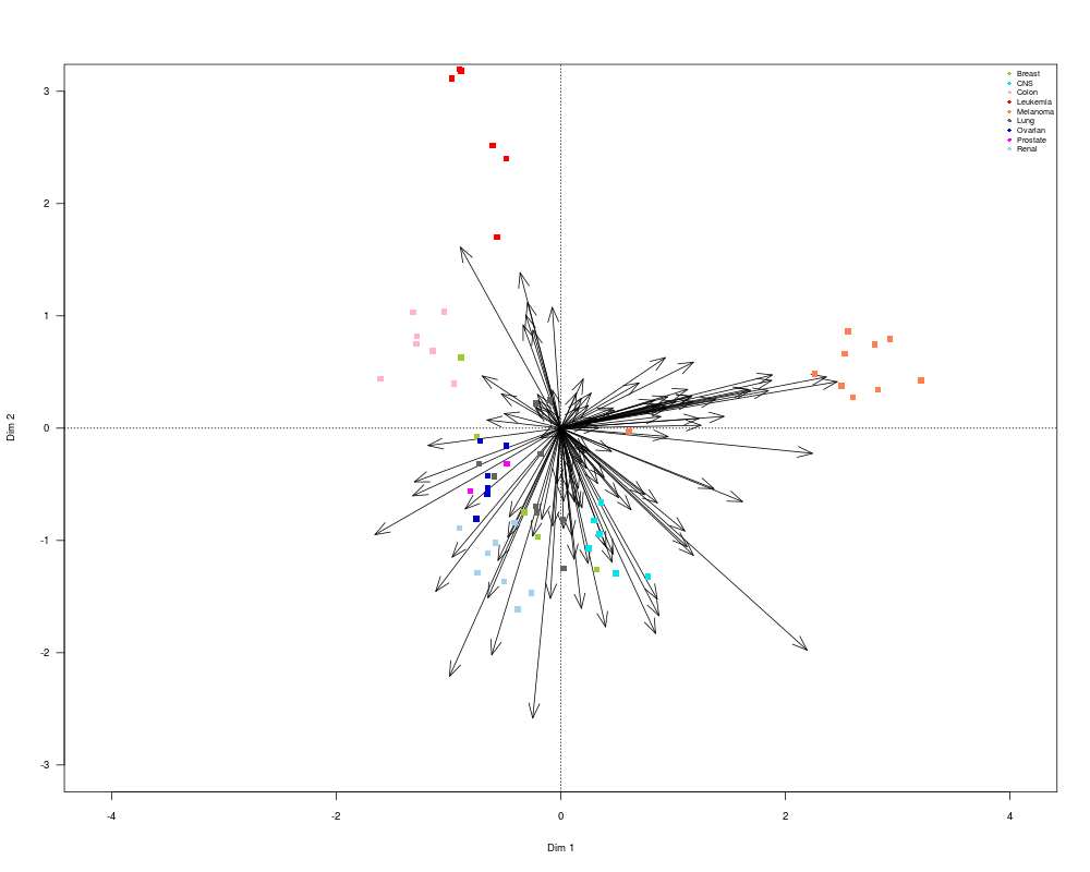
Biplot(M1,labelObs = FALSE,labelVars=FALSE,
colObs=Colores2,Type="SQRT",las=1,cex.axis=0.8,
cex.lab=0.8,xlimi=c(-3,3),ylimi=c(-3,3))
legend("topright",unique(Colores1),col=unique(Colores2),
bty="n",pch=16,cex=0.6)
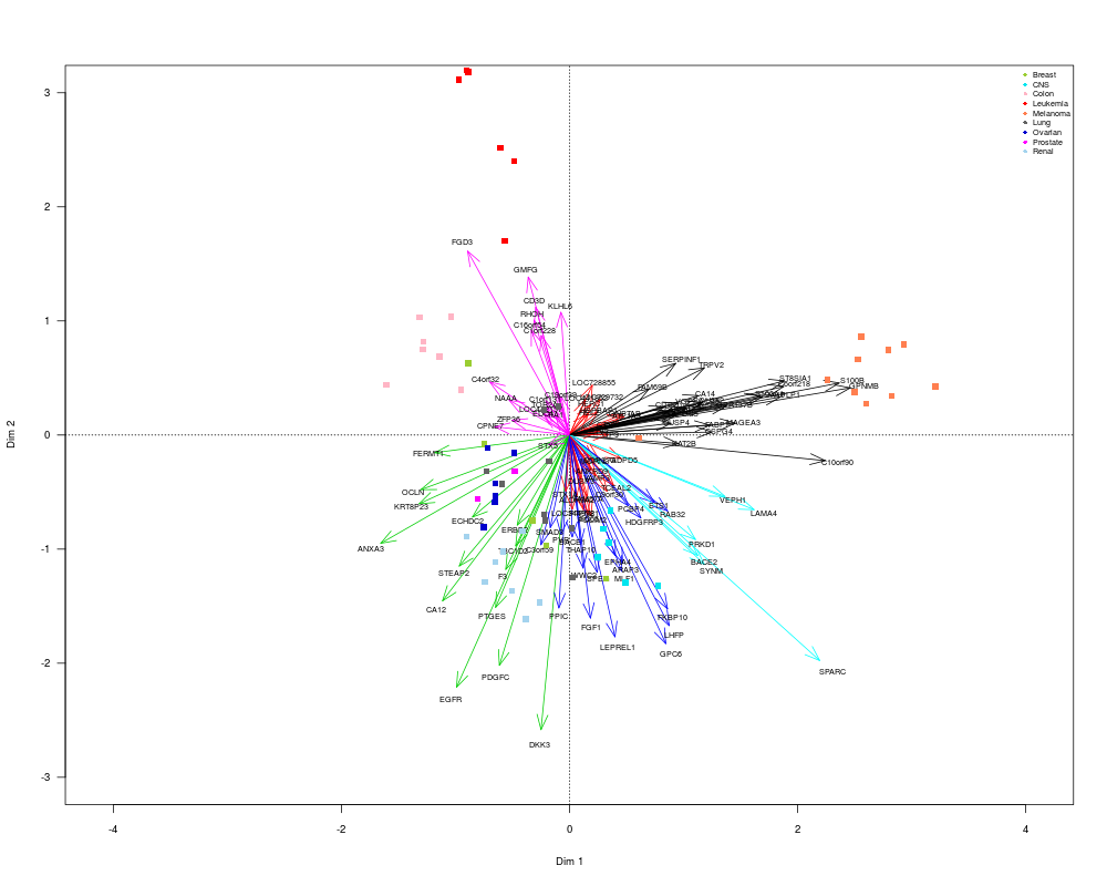
Biplot(M1,labelObs = FALSE,labelVars=TRUE,colObs=Colores2,
Type="SQRT",las=1,cex.axis=0.8,cex.lab=0.8,xlimi=c(-3,3),
ylimi=c(-3,3),Groups=TRUE,NGroups=6)
legend("topright",unique(Colores1),col=unique(Colores2),
bty="n",pch=16,cex=0.6)
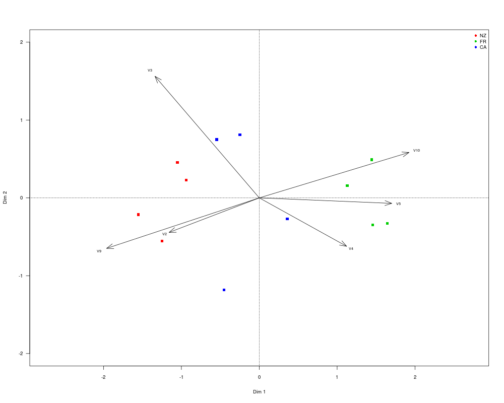
data(winesassesors)
Z3<-DiStatis(winesassesors)
M3<-SelectVar(Z3,Crit="R2-Adj")
Col1<-c(rep("NZ",4),rep("FR",4),rep("CA",4))
Col2<-c(rep(2,4),rep(3,4),rep(4,4))
Biplot(M3,labelObs=FALSE,labelVars=TRUE,colObs=Col2,
Type="SQRT",xlimi=c(-2,2),ylimi=c(-2,2),las=1,cex.axis=0.8,
cex.lab=0.8)
legend("topright",unique(Col1),col=unique(Col2),bty="n",pch=16,cex=0.8)
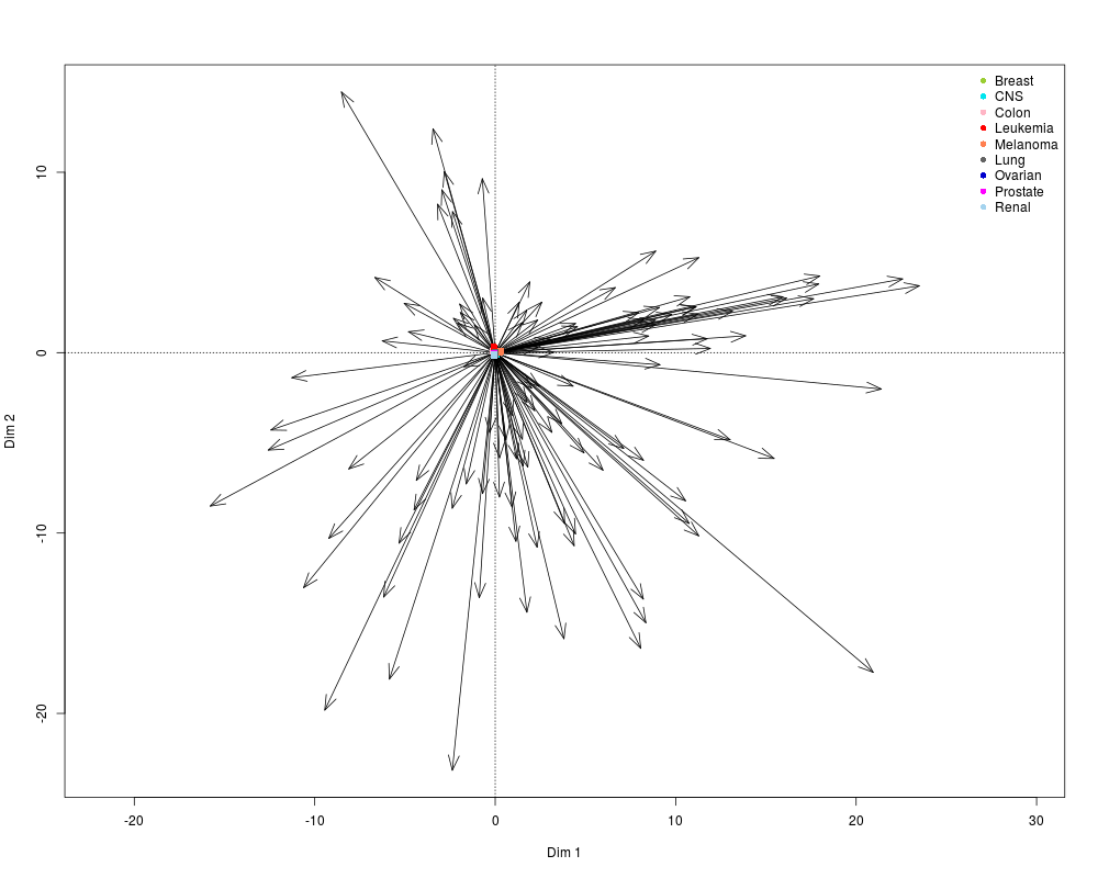
Biplot(M1,labelObs = FALSE,labelVars=FALSE,colObs=Colores2,
Type="CMP")
legend("topright",unique(Colores1),
col=unique(Colores2),bty="n",pch=16,cex=1)

}

Results


R version 3.3.1 (2016-06-21) -- "Bug in Your Hair"
Copyright (C) 2016 The R Foundation for Statistical Computing
Platform: x86_64-pc-linux-gnu (64-bit)

R is free software and comes with ABSOLUTELY NO WARRANTY.
You are welcome to redistribute it under certain conditions.
Type 'license()' or 'licence()' for distribution details.

R is a collaborative project with many contributors.
Type 'contributors()' for more information and
'citation()' on how to cite R or R packages in publications.

Type 'demo()' for some demos, 'help()' for on-line help, or
'help.start()' for an HTML browser interface to help.
Type 'q()' to quit R.

> library(kimod)
> png(filename="/home/ddbj/snapshot/RGM3/R_BC/result/kimod/SelectVar-Biplot.Rd_%03d_medium.png", width=480, height=480)
> ### Name: Biplot
> ### Title: Plot a 'Biplot' of a SelectVar class object
> ### Aliases: Biplot Biplot,SelectVar-method
> 
> ### ** Examples
> 
> {
+ data(NCI60Selec)
+ Z1<-DiStatis(NCI60Selec)
+ M1<-SelectVar(Z1,Crit="R2-Adj")
+ Colores1<-c(rep("Breast",5),rep("CNS",6),rep("Colon",7),
+ rep("Leukemia",6),rep("Melanoma",10),rep("Lung",9),
+ rep("Ovarian",7),rep("Prostate",2),rep("Renal",8))
+ Colores2<-c(rep(colors()[657],5),rep(colors()[637],6),
+ rep(colors()[537],7),rep(colors()[552],6),rep(colors()[57],10)
+ ,rep(colors()[300],9),rep(colors()[461],7),rep(colors()[450],2)
+ ,rep(colors()[432],8))
+ Biplot(M1,labelObs = FALSE,labelVars=FALSE,
+ colObs=Colores2,Type="SQRT",las=1,cex.axis=0.8,
+ cex.lab=0.8,xlimi=c(-3,3),ylimi=c(-3,3))
+ legend("topright",unique(Colores1),col=unique(Colores2),
+ bty="n",pch=16,cex=0.6)
+ Biplot(M1,labelObs = FALSE,labelVars=TRUE,colObs=Colores2,
+ Type="SQRT",las=1,cex.axis=0.8,cex.lab=0.8,xlimi=c(-3,3),
+ ylimi=c(-3,3),Groups=TRUE,NGroups=6)
+ legend("topright",unique(Colores1),col=unique(Colores2),
+ bty="n",pch=16,cex=0.6)
+ data(winesassesors)
+ Z3<-DiStatis(winesassesors)
+ M3<-SelectVar(Z3,Crit="R2-Adj")
+ Col1<-c(rep("NZ",4),rep("FR",4),rep("CA",4))
+ Col2<-c(rep(2,4),rep(3,4),rep(4,4))
+ Biplot(M3,labelObs=FALSE,labelVars=TRUE,colObs=Col2,
+ Type="SQRT",xlimi=c(-2,2),ylimi=c(-2,2),las=1,cex.axis=0.8,
+ cex.lab=0.8)
+ legend("topright",unique(Col1),col=unique(Col2),bty="n",pch=16,cex=0.8)
+ Biplot(M1,labelObs = FALSE,labelVars=FALSE,colObs=Colores2,
+ Type="CMP")
+ legend("topright",unique(Colores1),
+ col=unique(Colores2),bty="n",pch=16,cex=1)
+ 
+ }
The calculations were performed using the scalar product between the tables
The Projection of all variables will be made when the number of variables is less than 50
The calculations were performed using the scalar product between the tables
The Projection of all variables will be made when the number of variables is less than 50
> 
> 
> 
> 
> 
> dev.off()
null device 
          1 
>

Plot a Biplot of a SelectVar class object