R Graphical Manual

Browse All

Last data update: 2014.03.03

R: Empirical Bayes Statistics for Differential Expression under...

lapmix.Fit

R Documentation

Empirical Bayes Statistics for Differential Expression under Laplace Model

Description

Computes posterior odds of differential expression under the Laplace mixture model, with parameters estimated using an empirical Bayes approach.

Usage

lapmix.Fit(Y, asym=FALSE, fast=TRUE, two.step=TRUE, 
           w=0.1, V=10, beta=0, gamma=1, alpha=0.1)

Arguments

`Y`	data.frame or matrix containing the log relative expression levels, where each row represents a gene. Alternatively, a list of arrays of possibly different sizes, or an object of class `eSet` or `ExpressionSet`.
`asym`	indicates whether the asymmetric Laplace model is used rather than the symmetric one.
`fast`	indicates whether the 'fast' estimation method is used.
`two.step`	indicates whether the two-step estimation method is used; otherwise the marginal likelihood is maximised in one step.
`w,V,beta,gamma,alpha`	initial values given to the optimization algorithms for the estimation of the hyperparameters.

Details

This method fits the results of a microarray experiment to a Laplace mixture model. These results are assumed to take the form of normalized base 2 logarithm of the expression ratios. An empirical Bayes approach is used to estimate the hyperparameters of the model. The lap.lodds is sometimes known as the L-statistic (if the symmetric model is used) or the AL-statistic (if the asymmetric model is used). These statistics can be used to rank the genes according to the posterior odds of differential expression, via the routine laptopTable. They can be visualized using the lap.volcanoplot function.

If there are different numbers of replicates between genes, one may wish to write the data in a list of arrays. If a matrix representation is desired, one can stick in NaN's where appropriate.

The ‘fast’ estimation method ignores the integrals which cannot be computed with the t-distribution function. This method is suggested, since these problematic integrals are few and far between. The estimates are practically not affected, and we avoid the potential problems that arise when integrating numerically with the integrate function.

Value

`lap.lods`	numeric vector containing the posterior log-odds of differential expression
`prob`	numeric vector containing the posterior probabilities of differential expression
`med.number`	number of differentially expressed genes according to the median rule
`M`	numeric vector with average log fold changes within genes
`s_sq`	numeric vector with sample variances within genes
`nb.rep`	numeric vector with number of replicates within genes
`estimates`	list containing the empirical Bayes estimates of the hyperparameters
`code`	integer indicating why the likelihood optmization terminated, cf. `nlm` routine. There are two such indicators in the case of the two-step estimation.

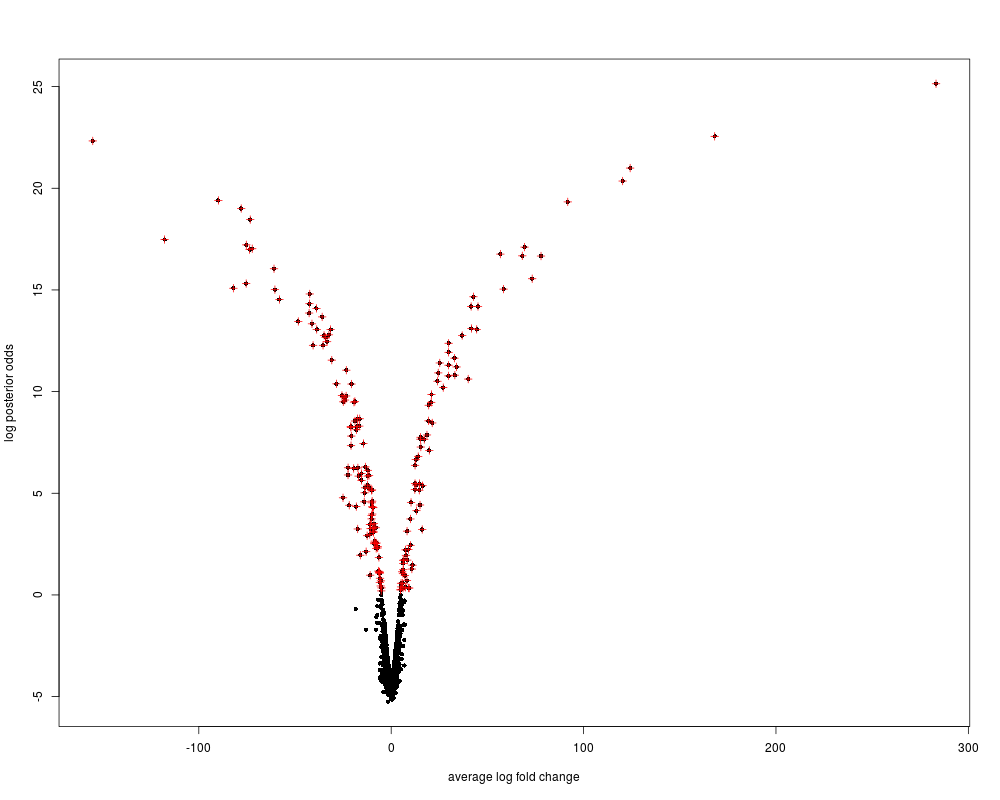
Author(s)

Yann Ruffieux

References

Bhowmick, D., Davison, A.C., and Goldstein, D.R. (2006). A Laplace mixture model for identification of differential expression in microarray experiments.

Examples

#  Simulate gene expression data under Laplace mixture model: 3000 genes with
#  4 duplicates each; one gene in ten is differentially expressed.

G <- 3000
Y <- NULL
sigma_sq <- 1/rgamma(G, shape=2.8, scale=0.04)
mu <- rexp(G, rate=1/(sigma_sq*1.2))-rexp(G, rate=1/(sigma_sq*1.2))
is.diff <- sample(c(0,1), replace=TRUE, prob=c(0.9,0.1), size=G)
mu <- mu*is.diff
for(g in 1:G)
	Y <- rbind(Y, rnorm(4,mu[g], sd=sqrt(sigma_sq[g])))

# with symmetric model
res <- lapmix.Fit(Y)
res$estimates
laptopTable(res, 20)
lap.volcanoplot(res, highlight=res$med.number)

# with asymmetric model
res2 <- lapmix.Fit(Y, asym=TRUE)
res2$estimates
laptopTable(res2, 20)
lap.volcanoplot(res2, highlight=res2$med.number)

Results


R version 3.3.1 (2016-06-21) -- "Bug in Your Hair"
Copyright (C) 2016 The R Foundation for Statistical Computing
Platform: x86_64-pc-linux-gnu (64-bit)

R is free software and comes with ABSOLUTELY NO WARRANTY.
You are welcome to redistribute it under certain conditions.
Type 'license()' or 'licence()' for distribution details.

R is a collaborative project with many contributors.
Type 'contributors()' for more information and
'citation()' on how to cite R or R packages in publications.

Type 'demo()' for some demos, 'help()' for on-line help, or
'help.start()' for an HTML browser interface to help.
Type 'q()' to quit R.

> library(lapmix)
> png(filename="/home/ddbj/snapshot/RGM3/R_BC/result/lapmix/lapmix.Fit.Rd_%03d_medium.png", width=480, height=480)
> ### Name: lapmix.Fit
> ### Title: Empirical Bayes Statistics for Differential Expression under
> ###   Laplace Model
> ### Aliases: lapmix.Fit
> ### Keywords: htest
> 
> ### ** Examples
> 
> #  Simulate gene expression data under Laplace mixture model: 3000 genes with
> #  4 duplicates each; one gene in ten is differentially expressed.
> 
> G <- 3000
> Y <- NULL
> sigma_sq <- 1/rgamma(G, shape=2.8, scale=0.04)
> mu <- rexp(G, rate=1/(sigma_sq*1.2))-rexp(G, rate=1/(sigma_sq*1.2))
> is.diff <- sample(c(0,1), replace=TRUE, prob=c(0.9,0.1), size=G)
> mu <- mu*is.diff
> for(g in 1:G)
+ 	Y <- rbind(Y, rnorm(4,mu[g], sd=sqrt(sigma_sq[g])))
> 
> # with symmetric model
> res <- lapmix.Fit(Y)
Warning messages:
1: In nlm(var.loglike, p = c(log(gamma), log(alpha)), s_sq = s_sq,  :
  NA/Inf replaced by maximum positive value
2: In nlm(var.loglike, p = c(log(gamma), log(alpha)), s_sq = s_sq,  :
  NA/Inf replaced by maximum positive value
3: In nlm(var.loglike, p = c(log(gamma), log(alpha)), s_sq = s_sq,  :
  NA/Inf replaced by maximum positive value
> res$estimates
$w
[1] 0.09170556

$V
[1] 1.26796

$beta
[1] 0

$gamma
[1] 2.58485

$alpha
[1] 0.04523682

> laptopTable(res, 20)
   gene          M log.odds
1  2399  311.69626 22.52015
2   209 -201.16717 20.40399
3  1792  139.89568 20.28531
4    61  -86.82083 18.82640
5   707 -109.64466 18.33879
6   924  -82.19704 18.13648
7  1131  -82.64860 17.65162
8   499  -84.98736 17.28920
9  2177   67.78158 17.20906
10 1597  -71.66394 17.18817
11 2388  -94.64714 16.80869
12 1815   66.11312 16.60589
13  714   64.42280 16.22412
14  484  -54.36724 15.53838
15  663   48.21172 15.32031
16 2443   71.56581 15.31171
17  316  -66.14542 15.08759
18  797   56.94083 14.94564
19 2613   93.35853 14.88660
20 1556   60.49439 14.88397
> lap.volcanoplot(res, highlight=res$med.number)
> 
> # with asymmetric model
> res2 <- lapmix.Fit(Y, asym=TRUE)
Warning messages:
1: In nlm(var.loglike, p = c(log(gamma), log(alpha)), s_sq = s_sq,  :
  NA/Inf replaced by maximum positive value
2: In nlm(var.loglike, p = c(log(gamma), log(alpha)), s_sq = s_sq,  :
  NA/Inf replaced by maximum positive value
3: In nlm(var.loglike, p = c(log(gamma), log(alpha)), s_sq = s_sq,  :
  NA/Inf replaced by maximum positive value
> res2$estimates
$w
[1] 0.0917798

$V
[1] 1.266259

$beta
[1] 0.02381835

$gamma
[1] 2.58485

$alpha
[1] 0.04523682

> laptopTable(res2, 20)
   gene          M log.odds
1  2399  311.69626 22.58385
2  1792  139.89568 20.36295
3   209 -201.16717 20.33948
4    61  -86.82083 18.73288
5   707 -109.64466 18.26878
6   924  -82.19704 18.05135
7  1131  -82.64860 17.57477
8  2177   67.78158 17.28475
9   499  -84.98736 17.21941
10 1597  -71.66394 17.10951
11 2388  -94.64714 16.75080
12 1815   66.11312 16.67457
13  714   64.42280 16.28922
14  484  -54.36724 15.46776
15  663   48.21172 15.38889
16 2443   71.56581 15.36206
17  316  -66.14542 15.03284
18  797   56.94083 15.00167
19 1556   60.49439 14.93680
20 2613   93.35853 14.92451
> lap.volcanoplot(res2, highlight=res2$med.number)
> 
> 
> 
> 
> 
> dev.off()
null device 
          1 
>