Supported by Dr. Osamu Ogasawara and  . . |
|
Last data update: 2014.03.03 |
Genuine Association of Gene Expression ProfilesDescriptionCalculates biological correlation between two gene expression profiles. Usagegenas(fit, coef=c(1,2), subset="all", plot=FALSE, alpha=0.4) Arguments
DetailsThe function estimates the biological correlation between two different contrasts in a linear model. By biological correlation, we mean the correlation that would exist between the log2-fold changes (logFC) for the two contrasts, if measurement error could be eliminated and the true log-fold-changes were known. This function is motivated by the fact that different contrasts for a linear model are often strongly correlated in a technical sense. For example, the estimated logFC for multiple treatment conditions compared back to the same control group will be positively correlated even in the absence of any biological effect. This function aims to separate the biological from the technical components of the correlation. The method is explained briefly in Majewski et al (2010) and in full detail in Phipson (2013). The The Value
NoteAs present, Author(s)Belinda Phipson and Gordon Smyth ReferencesMajewski, IJ, Ritchie, ME, Phipson, B, Corbin, J, Pakusch, M, Ebert, A, Busslinger, M, Koseki, H, Hu, Y, Smyth, GK, Alexander, WS, Hilton, DJ, and Blewitt, ME (2010). Opposing roles of polycomb repressive complexes in hematopoietic stem and progenitor cells. Blood 116, 731-739. http://www.bloodjournal.org/content/116/5/731 Phipson, B. (2013). Empirical Bayes modelling of expression profiles and their associations. PhD Thesis. University of Melbourne, Australia. http://repository.unimelb.edu.au/10187/17614 Ritchie, ME, Phipson, B, Wu, D, Hu, Y, Law, CW, Shi, W, and Smyth, GK (2015). limma powers differential expression analyses for RNA-sequencing and microarray studies. Nucleic Acids Research 43, e47. http://nar.oxfordjournals.org/content/43/7/e47 See Also
Examples
# Simulate gene expression data
# Three conditions (Control, A and B) and 1000 genes
ngene <- 1000
mu.A <- mu.B <- mu.ctrl <- rep(5,ngene)
# 200 genes are differentially expressed.
# All are up in condition A and down in B
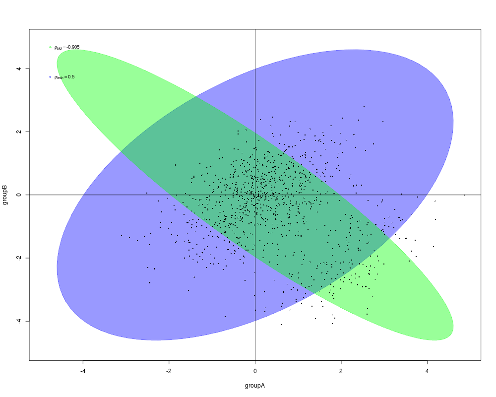
# so the biological correlation is negative.
mu.A[1:200] <- mu.ctrl[1:200]+2
mu.B[1:200] <- mu.ctrl[1:200]-2
# Two microarrays for each condition
mu <- cbind(mu.ctrl,mu.ctrl,mu.A,mu.A,mu.B,mu.B)
y <- matrix(rnorm(6000,mean=mu,sd=1),ngene,6)
# two experimental groups and one control group with two replicates each
group <- factor(c("Ctrl","Ctrl","A","A","B","B"), levels=c("Ctrl","A","B"))
design <- model.matrix(~group)
# fit a linear model
fit <- lmFit(y,design)
fit <- eBayes(fit)
# Estimate biological correlation between the logFC profiles
# for A-vs-Ctrl and B-vs-Ctrl
genas(fit, coef=c(2,3), plot=TRUE, subset="F")
Results
R version 3.3.1 (2016-06-21) -- "Bug in Your Hair"
Copyright (C) 2016 The R Foundation for Statistical Computing
Platform: x86_64-pc-linux-gnu (64-bit)

R is free software and comes with ABSOLUTELY NO WARRANTY.
You are welcome to redistribute it under certain conditions.
Type 'license()' or 'licence()' for distribution details.

R is a collaborative project with many contributors.
Type 'contributors()' for more information and
'citation()' on how to cite R or R packages in publications.

Type 'demo()' for some demos, 'help()' for on-line help, or
'help.start()' for an HTML browser interface to help.
Type 'q()' to quit R.

> library(limma)
> png(filename="/home/ddbj/snapshot/RGM3/R_BC/result/limma/genas.Rd_%03d_medium.png", width=480, height=480)
> ### Name: genas
> ### Title: Genuine Association of Gene Expression Profiles
> ### Aliases: genas genas
>
> ### ** Examples
>
> #  Simulate gene expression data
>
> #  Three conditions (Control, A and B) and 1000 genes
> ngene <- 1000
> mu.A <- mu.B <- mu.ctrl <- rep(5,ngene)
>
> #  200 genes are differentially expressed.
> #  All are up in condition A and down in B
> #  so the biological correlation is negative.
> mu.A[1:200] <- mu.ctrl[1:200]+2
> mu.B[1:200] <- mu.ctrl[1:200]-2
>
> #  Two microarrays for each condition
> mu <- cbind(mu.ctrl,mu.ctrl,mu.A,mu.A,mu.B,mu.B)
> y <- matrix(rnorm(6000,mean=mu,sd=1),ngene,6)
>
> # two experimental groups and one control group with two replicates each
> group <- factor(c("Ctrl","Ctrl","A","A","B","B"), levels=c("Ctrl","A","B"))
> design <- model.matrix(~group)
>
> # fit a linear model
> fit <- lmFit(y,design)
> fit <- eBayes(fit)
>
> #  Estimate biological correlation between the logFC profiles
> #  for A-vs-Ctrl and B-vs-Ctrl
> genas(fit, coef=c(2,3), plot=TRUE, subset="F")
$technical.correlation
[1] 0.5

$covariance.matrix
          [,1]      [,2]
[1,]  5.084251 -4.296684
[2,] -4.296684  4.735370

$biological.correlation
[1] -0.875675

$deviance
[1] 113.8391

$p.value
[1] 1.41322e-26

$n
[1] 179

>
>
>
>
>
> dev.off()
null device
          1
>
|