Supported by Dr. Osamu Ogasawara and  . . |
|
Last data update: 2014.03.03 |
Image Plot of Microarray StatisticsDescriptionCreates an image of colors or shades of gray that represent the values of a statistic for each spot on a spotted microarray. This function can be used to explore any spatial effects across the microarray. Usageimageplot(z, layout, low = NULL, high = NULL, ncolors = 123, zerocenter = NULL, zlim = NULL, mar=c(2,1,1,1), legend=TRUE, ...) Arguments
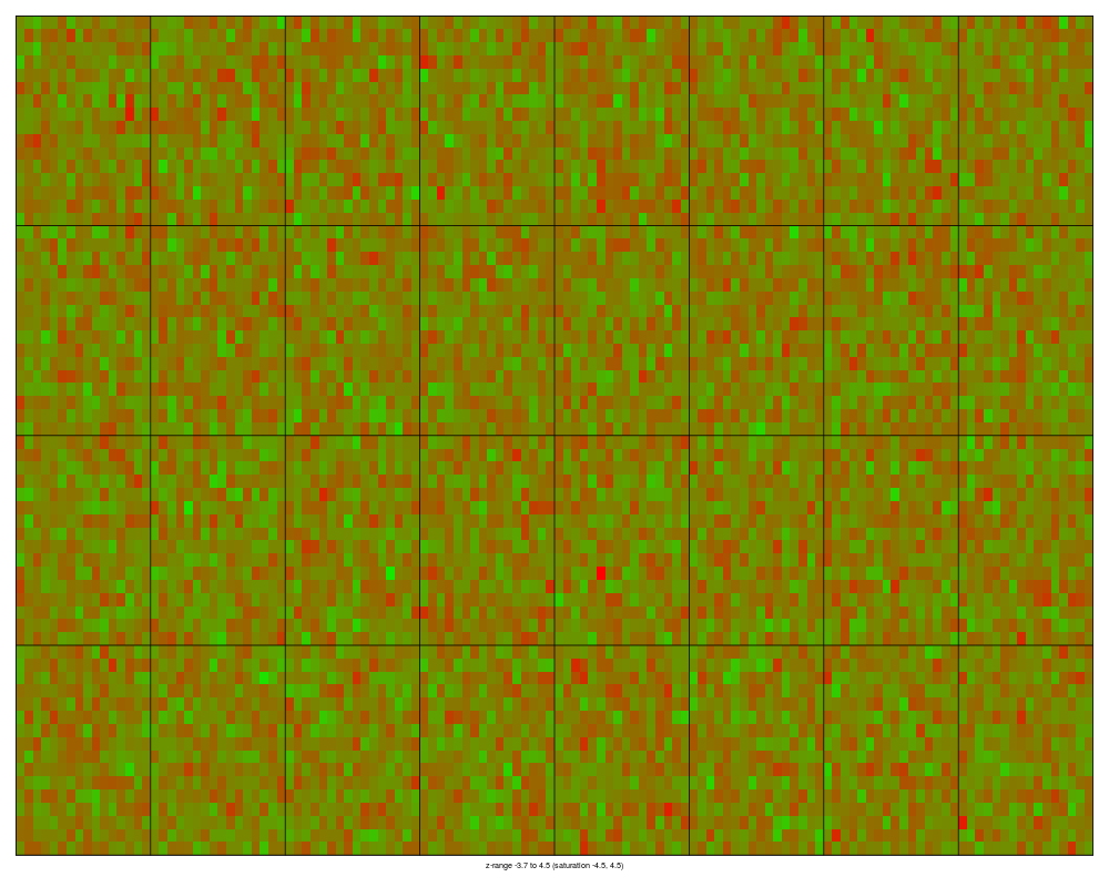
DetailsThis function may be used to plot the values of any spot-specific statistic, such as the log intensity ratio, background intensity or a quality measure such as spot size or shape. The image follows the layout of an actual microarray slide with the bottom left corner representing the spot (1,1,1,1). The color range is used to represent the range of values for the statistic. When this function is used to plot the red/green log-ratios, it is intended to be an in silico version of the classic false-colored red-yellow-green image of a scanned two-color microarray. This function is related to the earlier ValueAn plot is created on the current graphics device. Author(s)Gordon Smyth See Also
An overview of diagnostic functions available in LIMMA is given in 09.Diagnostics. ExamplesM <- rnorm(8*4*16*16) imageplot(M,layout=list(ngrid.r=8,ngrid.c=4,nspot.r=16,nspot.c=16)) Results
R version 3.3.1 (2016-06-21) -- "Bug in Your Hair"
Copyright (C) 2016 The R Foundation for Statistical Computing
Platform: x86_64-pc-linux-gnu (64-bit)

R is free software and comes with ABSOLUTELY NO WARRANTY.
You are welcome to redistribute it under certain conditions.
Type 'license()' or 'licence()' for distribution details.

R is a collaborative project with many contributors.
Type 'contributors()' for more information and
'citation()' on how to cite R or R packages in publications.

Type 'demo()' for some demos, 'help()' for on-line help, or
'help.start()' for an HTML browser interface to help.
Type 'q()' to quit R.

> library(limma)
> png(filename="/home/ddbj/snapshot/RGM3/R_BC/result/limma/imageplot.Rd_%03d_medium.png", width=480, height=480)
> ### Name: imageplot
> ### Title: Image Plot of Microarray Statistics
> ### Aliases: imageplot
> ### Keywords: hplot
>
> ### ** Examples
>
> M <- rnorm(8*4*16*16)
> imageplot(M,layout=list(ngrid.r=8,ngrid.c=4,nspot.r=16,nspot.c=16))
>
>
>
>
>
> dev.off()
null device
          1
>
|