Supported by Dr. Osamu Ogasawara and  . . |
|
Last data update: 2014.03.03 |
MA-Plot of Expression DataDescriptionCreates an MA-plot with color coding for control spots. Usage
## Default S3 method:
plotMA(object, array = 1, xlab = "Average log-expression",
       ylab = "Expression log-ratio (this sample vs others)",
       main = colnames(object)[array], status=NULL, ...)
## S3 method for class 'EList'
plotMA(object, array = 1, xlab = "Average log-expression",
       ylab = "Expression log-ratio (this sample vs others)",
       main = colnames(object)[array], status=object$genes$Status,
       zero.weights = FALSE, ...)
## S3 method for class 'RGList'
plotMA(object, array = 1, xlab = "A", ylab = "M",
       main = colnames(object)[array], status=object$genes$Status,
       zero.weights = FALSE, ...)
## S3 method for class 'MAList'
plotMA(object, array = 1, xlab = "A", ylab = "M",
       main = colnames(object)[array], status=object$genes$Status,
       zero.weights = FALSE, ...)
## S3 method for class 'MArrayLM'
plotMA(object, coef = ncol(object), xlab = "Average log-expression",
       ylab = "log-fold-change", main = colnames(object)[coef],
       status=object$genes$Status, zero.weights = FALSE, ...)
Arguments
DetailsAn MA-plot is a plot of log-intensity ratios (M-values) versus log-intensity averages (A-values). See Ritchie et al (2015) for a brief historical review. For two color data objects, a within-array MA-plot is produced with the M and A values computed from the two channels for the specified array.
This is the same as a mean-difference plot ( For single channel data objects, a between-array MA-plot is produced. An artificial array is produced by averaging all the arrays other than the array specified. A mean-difference plot is then producing from the specified array and the artificial array. Note that this procedure reduces to an ordinary mean-difference plot when there are just two arrays total. If The The See ValueA plot is created on the current graphics device. NoteThe Author(s)Gordon Smyth ReferencesRitchie, ME, Phipson, B, Wu, D, Hu, Y, Law, CW, Shi, W, and Smyth, GK (2015). limma powers differential expression analyses for RNA-sequencing and microarray studies. Nucleic Acids Research Volume 43, e47. http://nar.oxfordjournals.org/content/43/7/e47 See AlsoThe driver function for An overview of plot functions available in LIMMA is given in 09.Diagnostics. Examples
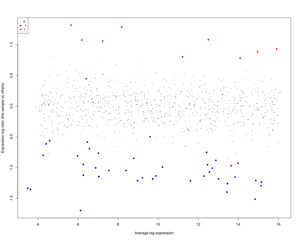
A <- runif(1000,4,16)
y <- A + matrix(rnorm(1000*3,sd=0.2),1000,3)
status <- rep(c(0,-1,1),c(950,40,10))
y[,1] <- y[,1] + status
plotMA(y, array=1, status=status, values=c(-1,1), hl.col=c("blue","red"))
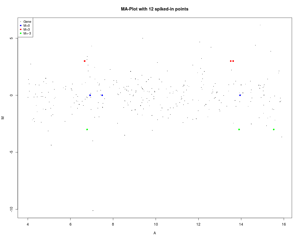
MA <- new("MAList")
MA$A <- runif(300,4,16)
MA$M <- rt(300,df=3)
# Spike-in values
MA$M[1:3] <- 0
MA$M[4:6] <- 3
MA$M[7:9] <- -3
status <- rep("Gene",300)
status[1:3] <- "M=0"
status[4:6] <- "M=3"
status[7:9] <- "M=-3"
values <- c("M=0","M=3","M=-3")
col <- c("blue","red","green")
plotMA(MA,main="MA-Plot with 12 spiked-in points",
status=status, values=values, hl.col=col)
# Same as above but setting graphical parameters as attributes
attr(status,"values") <- values
attr(status,"col") <- col
plotMA(MA, main="MA-Plot with 12 spiked-in points", status=status)
# Same as above but passing status as part of object
MA$genes$Status <- status
plotMA(MA, main="MA-Plot with 12 spiked-in points")
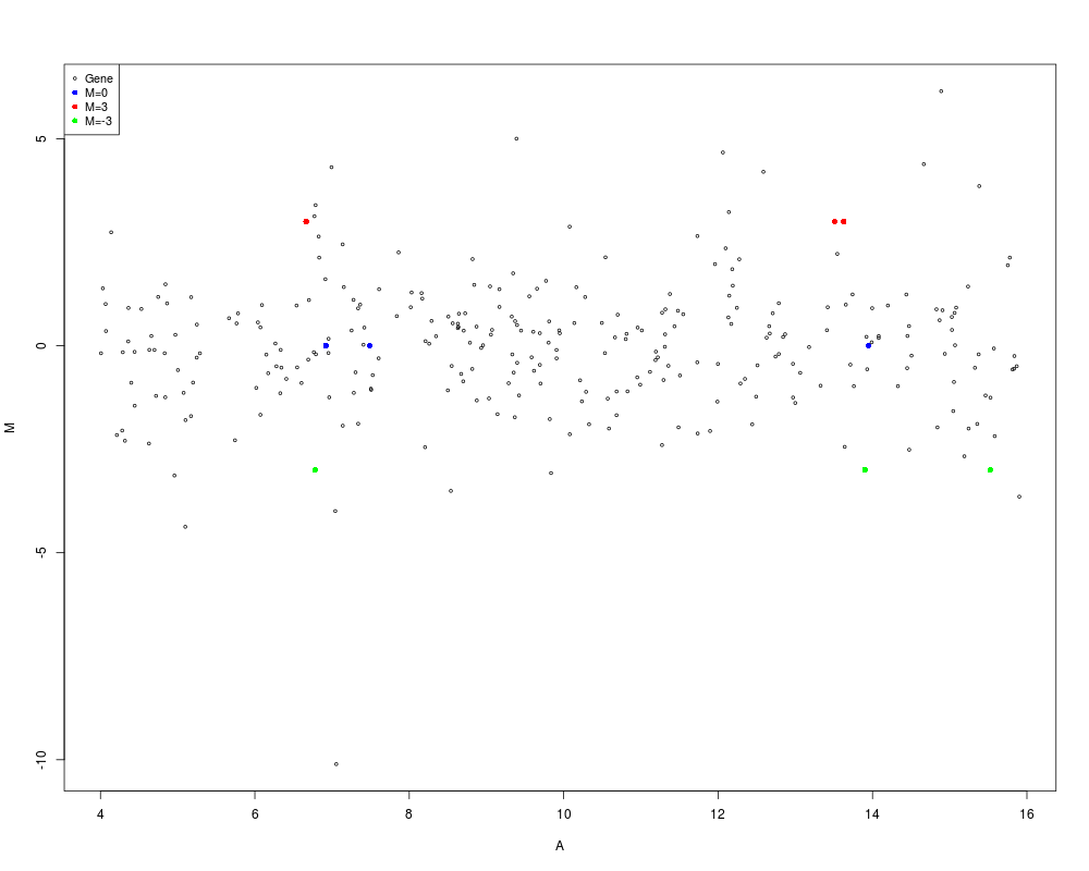
# Change settings for background points
MA$genes$Status <- status
plotMA(MA, bg.pch=1, bg.cex=0.5)
Results
R version 3.3.1 (2016-06-21) -- "Bug in Your Hair"
Copyright (C) 2016 The R Foundation for Statistical Computing
Platform: x86_64-pc-linux-gnu (64-bit)

R is free software and comes with ABSOLUTELY NO WARRANTY.
You are welcome to redistribute it under certain conditions.
Type 'license()' or 'licence()' for distribution details.

R is a collaborative project with many contributors.
Type 'contributors()' for more information and
'citation()' on how to cite R or R packages in publications.

Type 'demo()' for some demos, 'help()' for on-line help, or
'help.start()' for an HTML browser interface to help.
Type 'q()' to quit R.

> library(limma)
> png(filename="/home/ddbj/snapshot/RGM3/R_BC/result/limma/plotma.Rd_%03d_medium.png", width=480, height=480)
> ### Name: plotMA
> ### Title: MA-Plot of Expression Data
> ### Aliases: plotMA plotMA.RGList plotMA.MAList plotMA.EListRaw
> ###   plotMA.EList plotMA.MArrayLM plotMA.default
> ### Keywords: hplot
>
> ### ** Examples
>
> A <- runif(1000,4,16)
> y <- A + matrix(rnorm(1000*3,sd=0.2),1000,3)
> status <- rep(c(0,-1,1),c(950,40,10))
> y[,1] <- y[,1] + status
> plotMA(y, array=1, status=status, values=c(-1,1), hl.col=c("blue","red"))
>
> MA <- new("MAList")
> MA$A <- runif(300,4,16)
> MA$M <- rt(300,df=3)
>
> # Spike-in values
> MA$M[1:3] <- 0
> MA$M[4:6] <- 3
> MA$M[7:9] <- -3
>
> status <- rep("Gene",300)
> status[1:3] <- "M=0"
> status[4:6] <- "M=3"
> status[7:9] <- "M=-3"
> values <- c("M=0","M=3","M=-3")
> col <- c("blue","red","green")
>
> plotMA(MA,main="MA-Plot with 12 spiked-in points",
+        status=status, values=values, hl.col=col)
>
> #  Same as above but setting graphical parameters as attributes
> attr(status,"values") <- values
> attr(status,"col") <- col
> plotMA(MA, main="MA-Plot with 12 spiked-in points", status=status)
>
> #  Same as above but passing status as part of object
> MA$genes$Status <- status
> plotMA(MA, main="MA-Plot with 12 spiked-in points")
>
> #  Change settings for background points
> MA$genes$Status <- status
> plotMA(MA, bg.pch=1, bg.cex=0.5)
>
>
>
>
>
> dev.off()
null device
          1
>
|