Supported by Dr. Osamu Ogasawara and  . . |
|
Last data update: 2014.03.03 |
Lowess fit with weightingDescriptionFit robust lowess curves of degree 1 to weighted covariates and responses. Usage
weightedLowess(x, y, weights = rep(1, length(y)),
               delta=NULL, npts = 200, span = 0.3, iterations = 4)
Arguments
DetailsThis function extends the lowess algorithm to handle non-negative prior weights. These weights are
used during span calculations such that the span distance for each point must include the
specified proportion of all weights. They are also applied during weighted linear regression to
compute the fitted value (in addition to the tricube weights determined by For large vectors, running time is reduced by only performing locally weighted regression for several points. Fitted values for all points adjacent to the chosen points are computed by linear interpolation between the chosen points. For this purpose, the first and last points are always chosen. Note that the regression itself uses all (neighbouring) points. Points are defined as adjacent to a chosen point if the distance to the latter is positive and less
than Robustification is performed using the magnitude of the residuals. Residuals greater than 6 times the
median residual are assigned weights of zero. Otherwise, Tukey's biweight function is applied.
Weights are then used for weighted linear regression. Greater values of ValueA list of numeric vectors for the fitted responses, the residuals, the robustifying weights and the chosen delta. Author(s)Aaron Lun ReferencesCleveland, W.S. (1979). Robust Locally Weighted Regression and Smoothing Scatterplots. Journal of the American Statistical Association 74, 829-836. See Also
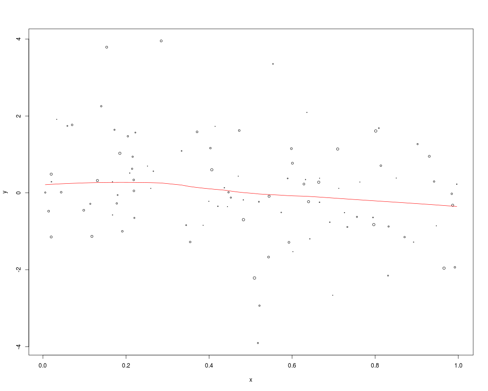
Examplesy <- rt(100,df=4) x <- runif(100) w <- runif(100) out <- weightedLowess(x, y, w, span=0.7) plot(x,y,cex=w) o <- order(x) lines(x[o],out$fitted[o],col="red") Results
R version 3.3.1 (2016-06-21) -- "Bug in Your Hair"
Copyright (C) 2016 The R Foundation for Statistical Computing
Platform: x86_64-pc-linux-gnu (64-bit)

R is free software and comes with ABSOLUTELY NO WARRANTY.
You are welcome to redistribute it under certain conditions.
Type 'license()' or 'licence()' for distribution details.

R is a collaborative project with many contributors.
Type 'contributors()' for more information and
'citation()' on how to cite R or R packages in publications.

Type 'demo()' for some demos, 'help()' for on-line help, or
'help.start()' for an HTML browser interface to help.
Type 'q()' to quit R.

> library(limma)
> png(filename="/home/ddbj/snapshot/RGM3/R_BC/result/limma/weightedLowess.Rd_%03d_medium.png", width=480, height=480)
> ### Name: weightedLoess
> ### Title: Lowess fit with weighting
> ### Aliases: weightedLowess
>
> ### ** Examples
>
> y <- rt(100,df=4)
> x <- runif(100)
> w <- runif(100)
> out <- weightedLowess(x, y, w, span=0.7)
> plot(x,y,cex=w)
> o <- order(x)
> lines(x[o],out$fitted[o],col="red")
>
>
>
>
>
> dev.off()
null device
          1
>
|