Estimate the copy number profile

Description

Function to estimate the copy number profile with a piecewise constant function using mBPCR. Eventually, it is possible to estimate the profile with a smoothing curve using either the Bayesian Regression Curve with K_2 (BRC with K_2) or the Bayesian Regression Curve Averaging over k (BRCAk). It is also possible to choose the estimator of the variance of the levels rhoSquare (i.e. either hat{ρ}_1^2 or hat{ρ}^2) and by default hat{ρ}_1^2 is used.

Usage

 computeMBPCR(y, kMax=50, nu=NULL, rhoSquare=NULL, sigmaSquare=NULL, typeEstRho=1, regr=NULL)

Arguments

Details

By default, the function estimates the copy number profile with mBPCR and estimating rhoSquare on the sample, using hat{ρ}_1^2. It is also possible to use hat{ρ}^2 as estimator of rhoSquare, by setting typeEstRho=0, or to directly set the value of the parameter.

The function gives also the possibility to estimate the profile with a Bayesian regression curve: if regr="BRC" the Bayesian Regression Curve with K_2 is computed (BRC with K_2), if regr="BRCAk" the Bayesian Regression Curve Averaging over k is computed (BRCAk).

Value

A list containing:

References

Rancoita, P. M. V., Hutter, M., Bertoni, F., Kwee, I. (2009). Bayesian DNA copy number analysis. BMC Bioinformatics 10: 10. http://www.idsia.ch/~paola/mBPCR

See Also

estProfileWithMBPCR, plotEstProfile, writeEstProfile, estGlobParam

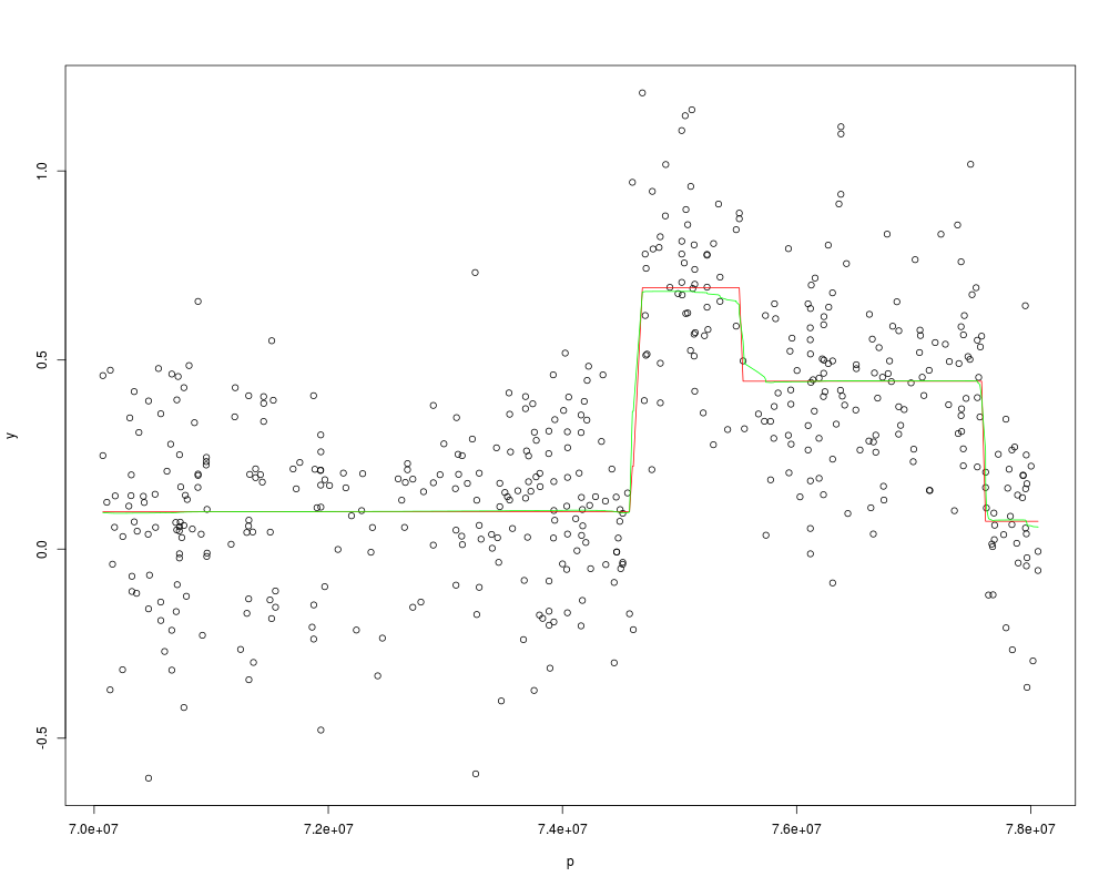
Examples

##import the 250K NSP data of chromosome 11 of cell line JEKO-1 
data(jekoChr11Array250Knsp)


##first example 
## we select a part of chromosome 11
y <- jekoChr11Array250Knsp$log2ratio[6400:6900]
p <- jekoChr11Array250Knsp$PhysicalPosition[6400:6900]
##we estimate the profile using the global parameters estimated on the whole genome
##the profile is estimated with mBPCR and with the Bayesian Regression Curve
results <- computeMBPCR(y, nu=-3.012772e-10, rhoSquare=0.0479, sigmaSquare=0.0699, regr="BRC")
plot(p, y)
points(p, results$estPC, type='l', col='red')
points(p, results$regrCurve,type='l', col='green')

###second example 
### we select a part of chromosome 11
#y <- jekoChr11Array250Knsp$log2ratio[10600:11600]
#p <- jekoChr11Array250Knsp$PhysicalPosition[10600:11600]
###we estimate the profile using the global parameters estimated on the whole genome
###the profile is estimated with mBPCR and with the Bayesian Regression Curve Ak
#results <- computeMBPCR(y, nu=-3.012772e-10, rhoSquare=0.0479, sigmaSquare=0.0699, regr="BRCAk")
#plot(p,y)
#points(p, results$estPC, type='l', col='red')
#points(p, results$regrCurve, type='l', col='green')

Results

R version 3.3.1 (2016-06-21) -- "Bug in Your Hair"
Copyright (C) 2016 The R Foundation for Statistical Computing
Platform: x86_64-pc-linux-gnu (64-bit)

R is free software and comes with ABSOLUTELY NO WARRANTY.
You are welcome to redistribute it under certain conditions.
Type 'license()' or 'licence()' for distribution details.

R is a collaborative project with many contributors.
Type 'contributors()' for more information and
'citation()' on how to cite R or R packages in publications.

Type 'demo()' for some demos, 'help()' for on-line help, or
'help.start()' for an HTML browser interface to help.
Type 'q()' to quit R.

> library(mBPCR)
Loading required package: oligoClasses
Welcome to oligoClasses version 1.34.0
Loading required package: SNPchip
Welcome to SNPchip version 2.18.0
> png(filename="/home/ddbj/snapshot/RGM3/R_BC/result/mBPCR/computeMBPCR.Rd_%03d_medium.png", width=480, height=480)
> ### Name: computeMBPCR
> ### Title: Estimate the copy number profile
> ### Aliases: computeMBPCR
> ### Keywords: regression smooth
> 
> ### ** Examples
> 
> ##import the 250K NSP data of chromosome 11 of cell line JEKO-1 
> data(jekoChr11Array250Knsp)
> 
> 
> ##first example 
> ## we select a part of chromosome 11
> y <- jekoChr11Array250Knsp$log2ratio[6400:6900]
> p <- jekoChr11Array250Knsp$PhysicalPosition[6400:6900]
> ##we estimate the profile using the global parameters estimated on the whole genome
> ##the profile is estimated with mBPCR and with the Bayesian Regression Curve
> results <- computeMBPCR(y, nu=-3.012772e-10, rhoSquare=0.0479, sigmaSquare=0.0699, regr="BRC")
Computation of log(A^0)
Computation of left and right recursions
Determination of PC Regression
Computation of Bayesian regression Curve
> plot(p, y)
> points(p, results$estPC, type='l', col='red')
> points(p, results$regrCurve,type='l', col='green')
> 
> ###second example 
> ### we select a part of chromosome 11
> #y <- jekoChr11Array250Knsp$log2ratio[10600:11600]
> #p <- jekoChr11Array250Knsp$PhysicalPosition[10600:11600]
> ###we estimate the profile using the global parameters estimated on the whole genome
> ###the profile is estimated with mBPCR and with the Bayesian Regression Curve Ak
> #results <- computeMBPCR(y, nu=-3.012772e-10, rhoSquare=0.0479, sigmaSquare=0.0699, regr="BRCAk")
> #plot(p,y)
> #points(p, results$estPC, type='l', col='red')
> #points(p, results$regrCurve, type='l', col='green')
> 
> 
> 
> 
> 
> 
> dev.off()
null device 
          1 
>