Supported by Dr. Osamu Ogasawara and  . . |
|
Last data update: 2014.03.03 |
Between group analysisDescriptionDiscrimination of samples using between group analysis as described by Culhane et al., 2002. Usage
bga(dataset, classvec, type = "coa", ...)
## S3 method for class 'bga'
plot(x, axis1=1, axis2=2, arraycol=NULL, genecol="gray25", nlab=10,
         genelabels= NULL, ...)
Arguments
Details
Between group analysis is a supervised method for sample discrimination and class prediction.
BGA is carried out by ordinating groups (sets of grouped microarray samples), that is,
groups of samples are projected into a reduced dimensional space. This is most easily
done using PCA or COA, of the group means. The choice of PCA, COA is defined by the parameter The user must define microarray sample groupings in advance. These groupings are defined using
the input Cross-validation and testing of bga results: bga results should be validated using one leave out jack-knife cross-validation using
Plotting and visualising bga results:
1D plots, show one axis only:
1D graphs can be plotted using 2D plots:
Use 3D plots:
3D graphs can be generated using Analysis of the distribution of variance among axes: It is important to know which cases (microarray samples) are discriminated by the axes.
The number of axes or principal components from a The distribution of variance among axes is described in the eigenvalues ($eig) of the Extracting list of top variables (genes): Use For more details see Culhane et al., 2002 and http://bioinf.ucd.ie/research/BGA. ValueA list with a class
Author(s)Aedin Culhane ReferencesCulhane AC, et al., 2002 Between-group analysis of microarray data. Bioinformatics. 18(12):1600-8. See AlsoSee Also Examples
data(khan)
if (require(ade4, quiet = TRUE)) {
khan.bga<-bga(khan$train, classvec=khan$train.classes)
}
khan.bga
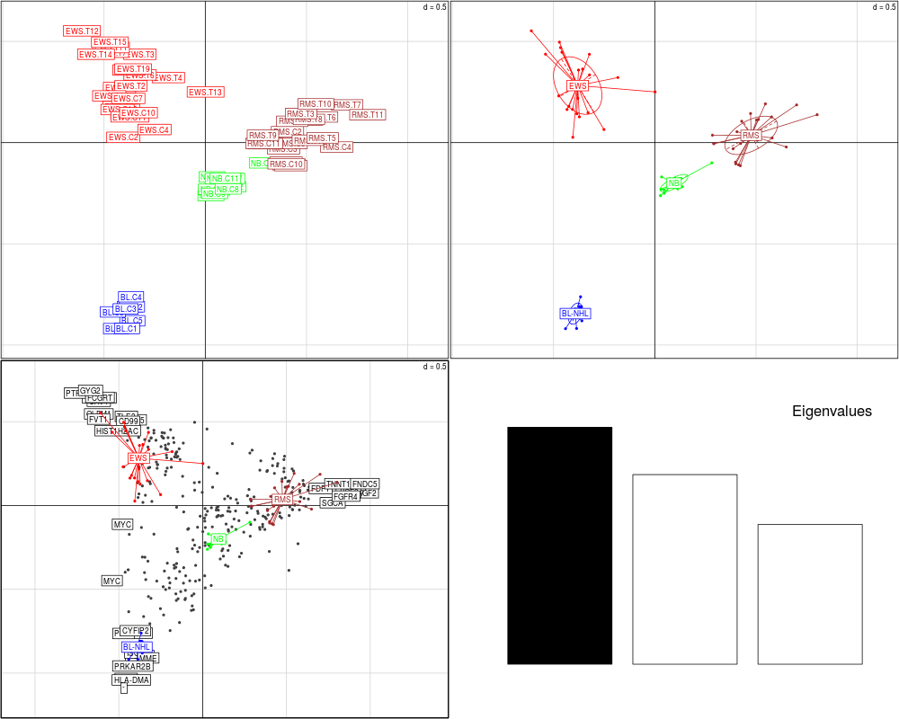
plot(khan.bga, genelabels=khan$annotation$Symbol)
# Provide a view of the principal components (axes) of the bga
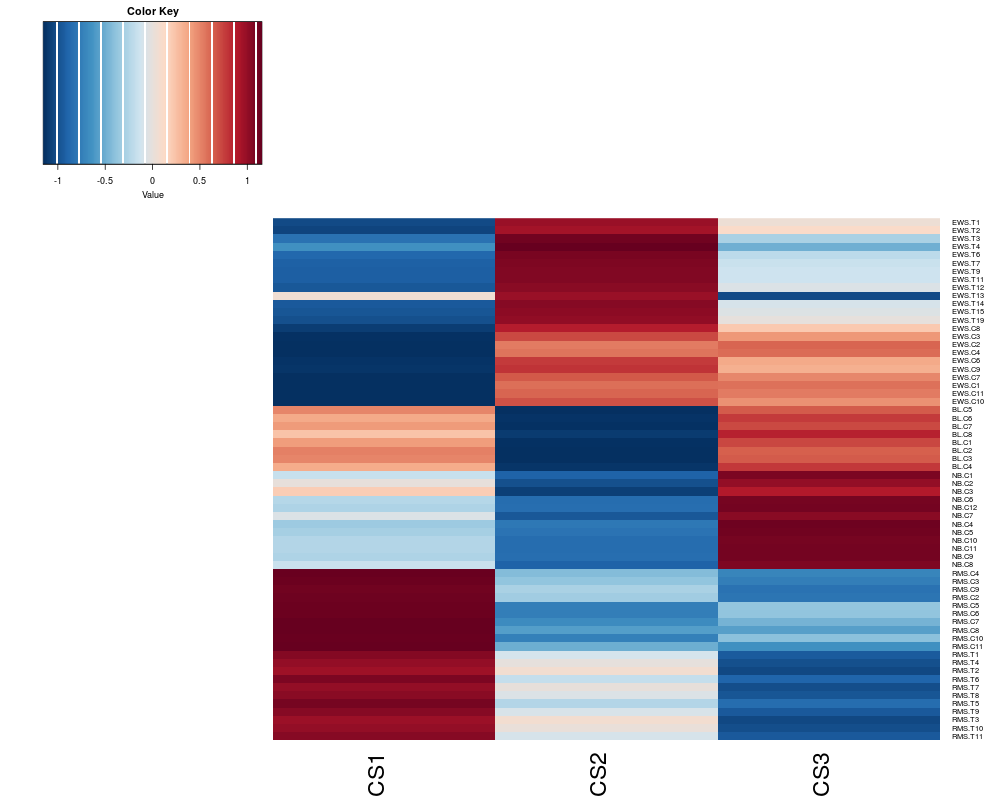
heatplot(khan.bga$bet$ls, dend="none")
Results
R version 3.3.1 (2016-06-21) -- "Bug in Your Hair"
Copyright (C) 2016 The R Foundation for Statistical Computing
Platform: x86_64-pc-linux-gnu (64-bit)

R is free software and comes with ABSOLUTELY NO WARRANTY.
You are welcome to redistribute it under certain conditions.
Type 'license()' or 'licence()' for distribution details.

R is a collaborative project with many contributors.
Type 'contributors()' for more information and
'citation()' on how to cite R or R packages in publications.

Type 'demo()' for some demos, 'help()' for on-line help, or
'help.start()' for an HTML browser interface to help.
Type 'q()' to quit R.

> library(made4)
Loading required package: ade4
Loading required package: RColorBrewer
Loading required package: gplots

Attaching package: 'gplots'

The following object is masked from 'package:stats':

    lowess

Loading required package: scatterplot3d
> png(filename="/home/ddbj/snapshot/RGM3/R_BC/result/made4/bga.Rd_%03d_medium.png", width=480, height=480)
> ### Name: bga
> ### Title: Between group analysis
> ### Aliases: bga plot.bga
> ### Keywords: manip multivariate
>
> ### ** Examples
>
> data(khan)
>
> if (require(ade4, quiet = TRUE)) {
+   khan.bga<-bga(khan$train, classvec=khan$train.classes)
+   }
>
> khan.bga
$ord
$ord
Duality diagramm
class: coa dudi
$call: dudi.coa(df = data.tr, scannf = FALSE, nf = ord.nf)

$nf: 63 axis-components saved
$rank: 63
eigen values: 0.1713 0.1383 0.1032 0.05995 0.04965 ...
  vector length mode    content
1 $cw    306    numeric column weights
2 $lw    64     numeric row weights
3 $eig   63     numeric eigen values

  data.frame nrow ncol content
1 $tab       64   306  modified array
2 $li        64   63   row coordinates
3 $l1        64   63   row normed scores
4 $co        306  63   column coordinates
5 $c1        306  63   column normed scores
other elements: N

$fac
 [1] EWS    EWS    EWS    EWS    EWS    EWS    EWS    EWS    EWS    EWS
[11] EWS    EWS    EWS    EWS    EWS    EWS    EWS    EWS    EWS    EWS
[21] EWS    EWS    EWS    BL-NHL BL-NHL BL-NHL BL-NHL BL-NHL BL-NHL BL-NHL
[31] BL-NHL NB     NB     NB     NB     NB     NB     NB     NB     NB
[41] NB     NB     NB     RMS    RMS    RMS    RMS    RMS    RMS    RMS
[51] RMS    RMS    RMS    RMS    RMS    RMS    RMS    RMS    RMS    RMS
[61] RMS    RMS    RMS    RMS
Levels: EWS BL-NHL NB RMS

attr(,"class")
[1] "coa" "ord"

$bet
Between analysis
call: bca.dudi(x = data.ord$ord, fac = classvec, scannf = FALSE, nf = nclasses -
    1)
class: between dudi

$nf (axis saved) : 3
$rank:  3
$ratio:  0.3599779

eigen values: 0.1522 0.1218 0.08981

  vector length mode    content
1 $eig   3      numeric eigen values
2 $lw    4      numeric group weigths
3 $cw    306    numeric col weigths

  data.frame nrow ncol content
1 $tab       4    306  array class-variables
2 $li        4    3    class coordinates
3 $l1        4    3    class normed scores
4 $co        306  3    column coordinates
5 $c1        306  3    column normed scores
6 $ls        64   3    row coordinates
7 $as        63   3    inertia axis onto between axis


$fac
 [1] EWS    EWS    EWS    EWS    EWS    EWS    EWS    EWS    EWS    EWS
[11] EWS    EWS    EWS    EWS    EWS    EWS    EWS    EWS    EWS    EWS
[21] EWS    EWS    EWS    BL-NHL BL-NHL BL-NHL BL-NHL BL-NHL BL-NHL BL-NHL
[31] BL-NHL NB     NB     NB     NB     NB     NB     NB     NB     NB
[41] NB     NB     NB     RMS    RMS    RMS    RMS    RMS    RMS    RMS
[51] RMS    RMS    RMS    RMS    RMS    RMS    RMS    RMS    RMS    RMS
[61] RMS    RMS    RMS    RMS
Levels: EWS BL-NHL NB RMS

attr(,"class")
[1] "coa" "bga"
> plot(khan.bga, genelabels=khan$annotation$Symbol)
>
> # Provide a view of the principal components (axes) of the bga
> heatplot(khan.bga$bet$ls, dend="none")
[1] "Data (original) range:  -0.92 0.8"
[1] "Data (scale) range:  -1.15 1.15"
[1] "Data scaled to range:  -1.15 1.15"
>
>
>
>
>
> dev.off()
null device
          1
>
|