Supported by Dr. Osamu Ogasawara and  . . |
|
Last data update: 2014.03.03 |
Coinertia analysis: Explore the covariance between two datasetsDescriptionPerforms CIA on two datasets as described by Culhane et al., 2003. Used for meta-analysis of two or more datasets. Usage
cia(df1, df2, cia.nf=2, cia.scan=FALSE, nsc=TRUE,...)
## S3 method for class 'cia'
plot(x, nlab = 10, axis1 = 1, axis2 = 2, genecol = "gray25",
         genelabels1 = rownames(ciares$co), genelabels2 = rownames(ciares$li), ...)
Arguments
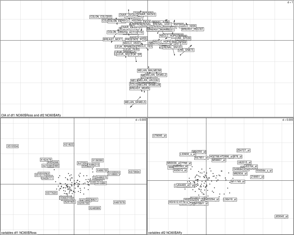
DetailsCIA has been successfully applied to the cross-platform comparison (meta-analysis) of microarray gene expression datasets (Culhane et al., 2003). Please refer to this paper and the vignette for help in interpretation of the output from CIA. Co-inertia analysis (CIA) is a multivariate method that identifies trends or co-relationships
in multiple datasets which contain the same samples. That is the rows or columns of the matrix have to
be weighted similarly and thus must be "matchable". In CIA simultaneously finds ordinations (dimension reduction diagrams) from the datasets that are most similar. It does this by finding successive axes from the two datasets with maximum covariance. CIA can be applied to datasets where the number of variables (genes) far exceeds the number of samples (arrays) such is the case with microarray analyses.
In the paper by Culhane et al., 2003, the datasets df1 and df2 are transformed using COA and Row weighted COA respectively, before coinertia analysis. It is now recommended to perform non symmetric correspondence analysis (NSC) rather than correspondence analysis (COA) on both datasets. The RV coefficient In the results, in the object Plotting and visualising cia results
The first plot uses The second two plots call Please refer to the help on ValueAn object of the class
Author(s)Aedin Culhane ReferencesCulhane AC, et al., 2003 Cross platform comparison and visualisation of gene expression data using co-inertia analysis. BMC Bioinformatics. 4:59 See AlsoSee also Examples
data(NCI60)
print("This will take a few minutes, please wait...")
if (require(ade4, quiet = TRUE)) {
# Example data are "G1_Ross_1375.txt" and "G5_Affy_1517.txt"
coin <- cia(NCI60$Ross, NCI60$Affy)
}
attach(coin)
summary(coin)
summary(coin$coinertia)
# $coinertia$RV will give the RV-coefficient, the greater (scale 0-1) the better
cat(paste("The RV coefficient is a measure of global similarity between the datasets.\n",
"The two datasets analysed are very similar. ",
"The RV coefficient of this coinertia analysis is: ", coin$coinertia$RV,"\n", sep= ""))
plot(coin)
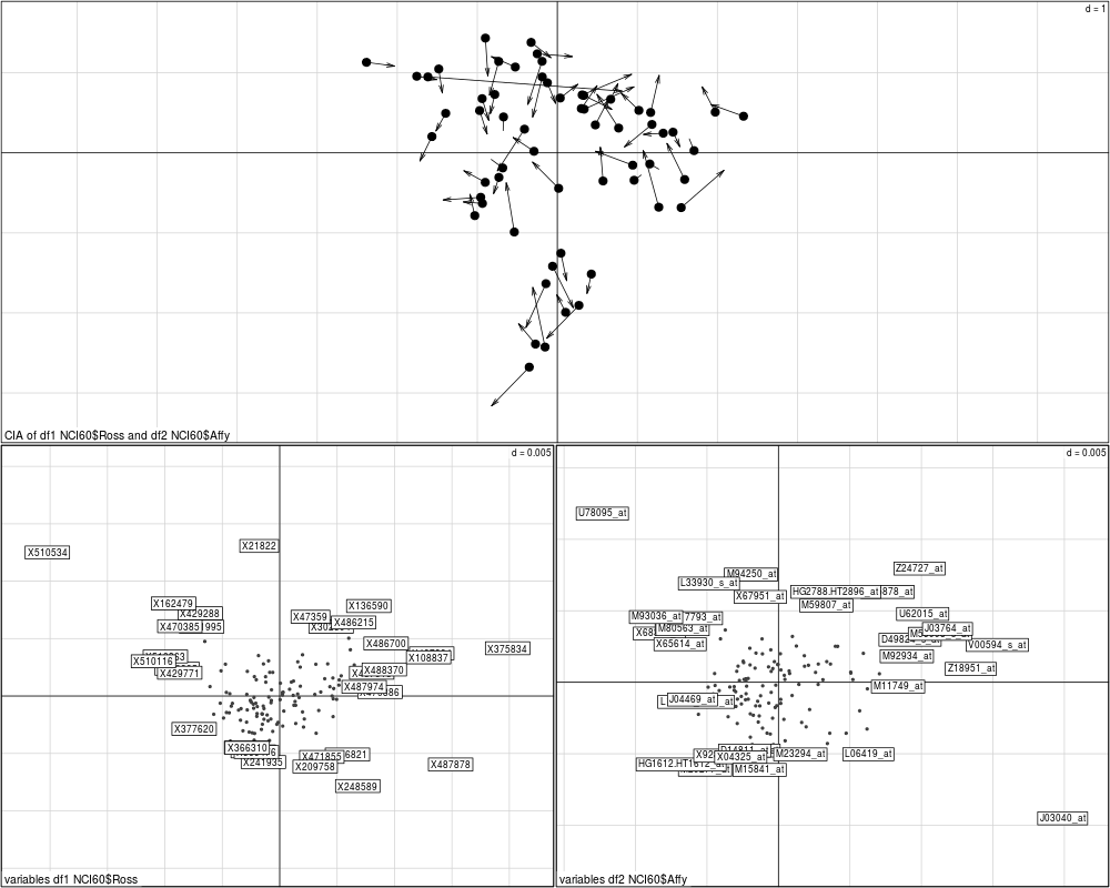
plot(coin, classvec=NCI60$classes[,2], clab=0, cpoint=3)
Results
R version 3.3.1 (2016-06-21) -- "Bug in Your Hair"
Copyright (C) 2016 The R Foundation for Statistical Computing
Platform: x86_64-pc-linux-gnu (64-bit)

R is free software and comes with ABSOLUTELY NO WARRANTY.
You are welcome to redistribute it under certain conditions.
Type 'license()' or 'licence()' for distribution details.

R is a collaborative project with many contributors.
Type 'contributors()' for more information and
'citation()' on how to cite R or R packages in publications.

Type 'demo()' for some demos, 'help()' for on-line help, or
'help.start()' for an HTML browser interface to help.
Type 'q()' to quit R.

> library(made4)
Loading required package: ade4
Loading required package: RColorBrewer
Loading required package: gplots

Attaching package: 'gplots'

The following object is masked from 'package:stats':

    lowess

Loading required package: scatterplot3d
> png(filename="/home/ddbj/snapshot/RGM3/R_BC/result/made4/cia.Rd_%03d_medium.png", width=480, height=480)
> ### Name: cia
> ### Title: Coinertia analysis: Explore the covariance between two datasets
> ### Aliases: cia plot.cia
> ### Keywords: multivariate hplot
>
> ### ** Examples
>
> data(NCI60)
> print("This will take a few minutes, please wait...")
[1] "This will take a few minutes, please wait..."
>
> if (require(ade4, quiet = TRUE)) {
+ 	# Example data are "G1_Ross_1375.txt" and "G5_Affy_1517.txt"
+ 	coin <- cia(NCI60$Ross, NCI60$Affy)
+ }
> attach(coin)
> summary(coin)
          Length Class     Mode
call       3     -none-    call
coinertia 18     coinertia list
coa1      11     transpo   list
coa2      11     transpo   list
> summary(coin$coinertia)
Coinertia analysis

Class: coinertia dudi
Call: coinertia(dudiX = coa1, dudiY = coa2, scannf = cia.scan, nf = cia.nf)

Total inertia: 4.876e-05

Eigenvalues:
      Ax1       Ax2       Ax3       Ax4       Ax5
2.266e-05 9.904e-06 4.342e-06 2.335e-06 1.576e-06

Projected inertia (%):
    Ax1     Ax2     Ax3     Ax4     Ax5
 46.476  20.312   8.904   4.789   3.233

Cumulative projected inertia (%):
    Ax1   Ax1:2   Ax1:3   Ax1:4   Ax1:5
  46.48   66.79   75.69   80.48   83.71

(Only 5 dimensions (out of 59) are shown)

Eigenvalues decomposition:
           eig       covar        sdX        sdY      corr
1 2.266249e-05 0.004760514 0.08187720 0.06339248 0.9171769
2 9.904435e-06 0.003147131 0.06862156 0.04851708 0.9452782

Inertia & coinertia X (coa1):
       inertia         max     ratio
1  0.006703875 0.007109399 0.9429596
12 0.011412793 0.011693125 0.9760259

Inertia & coinertia Y (coa2):
       inertia         max     ratio
1  0.004018607 0.004184413 0.9603752
12 0.006372514 0.006530483 0.9758105

RV:
 0.7859656
> # $coinertia$RV will give the RV-coefficient, the greater (scale 0-1) the better
> cat(paste("The RV coefficient is a measure of global similarity between the datasets.\n",
+ "The two datasets analysed are very similar. ",
+ "The RV coefficient of this coinertia analysis is: ", coin$coinertia$RV,"\n", sep= ""))
The RV coefficient is a measure of global similarity between the datasets.
The two datasets analysed are very similar. The RV coefficient of this coinertia analysis is: 0.785965616408393
> plot(coin)
> plot(coin, classvec=NCI60$classes[,2], clab=0, cpoint=3)
>
>
>
>
>
> dev.off()
null device
          1
>
|