Ordination

Description

Run principal component analysis, correspondence analysis or non-symmetric correspondence analysis on gene expression data

Usage

ord(dataset, type="coa", classvec=NULL,ord.nf=NULL, trans=FALSE, ...)
## S3 method for class 'ord'
plot(x, axis1=1, axis2=2, arraycol=NULL, genecol="gray25", nlab=10, genelabels= NULL, arraylabels=NULL,classvec=NULL, ...)

Arguments

Details

ord calls either dudi.pca, dudi.coa or dudi.nsc on the input dataset. The input format of the dataset is verified using array2ade4.

If the user defines microarray sample groupings, these are colours on plots produced by plot.ord.

Plotting and visualising bga results:

2D plots: plotarrays to draw an xy plot of cases ($ls). plotgenes, is used to draw an xy plot of the variables (genes).

3D plots: 3D graphs can be generated using do3D and html3D. html3D produces a web page in which a 3D plot can be interactively rotated, zoomed, and in which classes or groups of cases can be easily highlighted.

1D plots, show one axis only: 1D graphs can be plotted using graph1D. graph1D can be used to plot either cases (microarrays) or variables (genes) and only requires a vector of coordinates ($li, $co)

Analysis of the distribution of variance among axes:

The number of axes or principal components from a ord will equal nrow the number of rows, or the ncol, number of columns of the dataset (whichever is less).

The distribution of variance among axes is described in the eigenvalues ($eig) of the ord analysis. These can be visualised using a scree plot, using scatterutil.eigen as it done in plot.ord. It is also useful to visualise the principal components from a using a ord or principal components analysis dudi.pca, or correspondence analysis dudi.coa using a heatmap. In MADE4 the function heatplot will plot a heatmap with nicer default colours.

Extracting list of top variables (genes):

Use topgenes to get list of variables or cases at the ends of axes. It will return a list of the top n variables (by default n=5) at the positive, negative or both ends of an axes. sumstats can be used to return the angle (slope) and distance from the origin of a list of coordinates.

Value

A list with a class ord containing:

Author(s)

Aedin Culhane

See Also

See Also dudi.pca, dudi.coa or dudi.nsc, bga,

Examples

data(khan)

if (require(ade4, quiet = TRUE)) {
  khan.coa<-ord(khan$train, classvec=khan$train.classes, type="coa")  
}

khan.coa
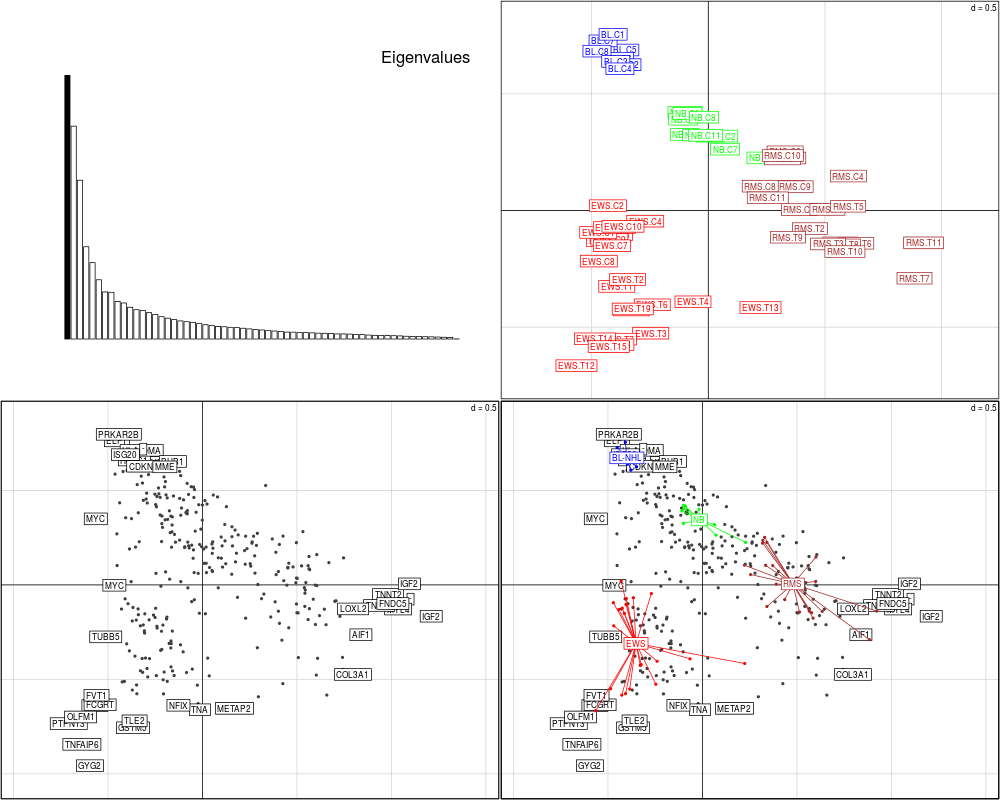
plot(khan.coa, genelabels=khan$annotation$Symbol)
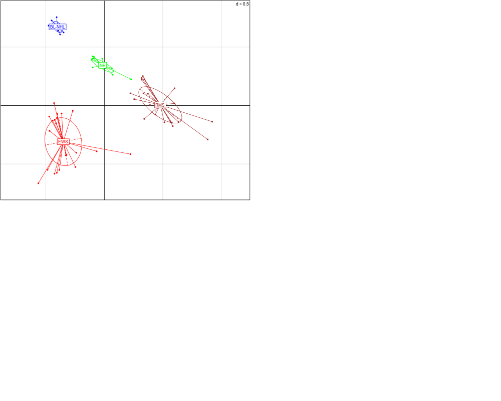
plotarrays(khan.coa)
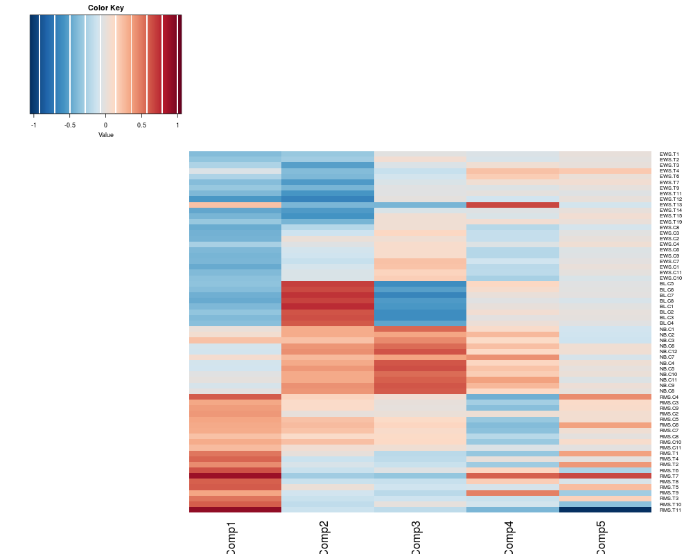
# Provide a view of the first 5 principal components (axes) of the correspondence analysis
heatplot(khan.coa$ord$co[,1:5], dend="none",dualScale=FALSE)

Results

R version 3.3.1 (2016-06-21) -- "Bug in Your Hair"
Copyright (C) 2016 The R Foundation for Statistical Computing
Platform: x86_64-pc-linux-gnu (64-bit)

R is free software and comes with ABSOLUTELY NO WARRANTY.
You are welcome to redistribute it under certain conditions.
Type 'license()' or 'licence()' for distribution details.

R is a collaborative project with many contributors.
Type 'contributors()' for more information and
'citation()' on how to cite R or R packages in publications.

Type 'demo()' for some demos, 'help()' for on-line help, or
'help.start()' for an HTML browser interface to help.
Type 'q()' to quit R.

> library(made4)
Loading required package: ade4
Loading required package: RColorBrewer
Loading required package: gplots

Attaching package: 'gplots'

The following object is masked from 'package:stats':

    lowess

Loading required package: scatterplot3d
> png(filename="/home/ddbj/snapshot/RGM3/R_BC/result/made4/ord.Rd_%03d_medium.png", width=480, height=480)
> ### Name: ord
> ### Title: Ordination
> ### Aliases: ord plot.ord
> ### Keywords: manip multivariate
> 
> ### ** Examples
> 
> data(khan)
> 
> if (require(ade4, quiet = TRUE)) {
+   khan.coa<-ord(khan$train, classvec=khan$train.classes, type="coa")  
+ }
> 
> khan.coa
$ord
Duality diagramm
class: coa dudi
$call: dudi.coa(df = data.tr, scannf = FALSE, nf = ord.nf)

$nf: 63 axis-components saved
$rank: 63
eigen values: 0.1713 0.1383 0.1032 0.05995 0.04965 ...
  vector length mode    content       
1 $cw    64     numeric column weights
2 $lw    306    numeric row weights   
3 $eig   63     numeric eigen values  

  data.frame nrow ncol content             
1 $tab       306  64   modified array      
2 $li        306  63   row coordinates     
3 $l1        306  63   row normed scores   
4 $co        64   63   column coordinates  
5 $c1        64   63   column normed scores
other elements: N 

$fac
 [1] EWS    EWS    EWS    EWS    EWS    EWS    EWS    EWS    EWS    EWS   
[11] EWS    EWS    EWS    EWS    EWS    EWS    EWS    EWS    EWS    EWS   
[21] EWS    EWS    EWS    BL-NHL BL-NHL BL-NHL BL-NHL BL-NHL BL-NHL BL-NHL
[31] BL-NHL NB     NB     NB     NB     NB     NB     NB     NB     NB    
[41] NB     NB     NB     RMS    RMS    RMS    RMS    RMS    RMS    RMS   
[51] RMS    RMS    RMS    RMS    RMS    RMS    RMS    RMS    RMS    RMS   
[61] RMS    RMS    RMS    RMS   
Levels: EWS BL-NHL NB RMS

attr(,"class")
[1] "coa" "ord"
> plot(khan.coa, genelabels=khan$annotation$Symbol)
> plotarrays(khan.coa)
> # Provide a view of the first 5 principal components (axes) of the correspondence analysis
> heatplot(khan.coa$ord$co[,1:5], dend="none",dualScale=FALSE)
> 
> 
> 
> 
> 
> dev.off()
null device 
          1 
>