Summary statistics on xy co-ordinates, returns the slopes and distance from origin of each co-ordinate.

Description

Given a data.frame or matrix containing xy coordinates, it returns the slope and distance from origin of each coordinate.

Usage

sumstats(array, xax = 1, yax = 2)

Arguments

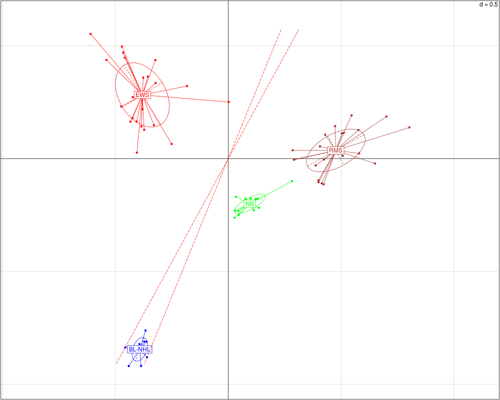
Details

In PCA or COA, the variables (upregulated genes) that are most associated with a case (microarray sample), are those that are projected in the same direction from the origin.

Variables or cases that have a greater contribution to the variance in the data are projected further from the origin in PCA. Equally variables and cases with the strong association have a high chi-square value, and are projected with greater distance from the origin in COA, See a description from Culhane et al., 2002 for more details.

Although the projection of co-ordinates are best visualised on an xy plot, sumstats returns the slope and distance from origin of each x,y coordinate in a matrix.

Value

A matrix (ncol=3) containing

   slope 
   angle (in degrees) 
   distance from origin 

of each x,y coordinates in a matrix.

Author(s)

Aedin Culhane

Examples

data(khan)

if (require(ade4, quiet = TRUE)) {

khan.bga<-bga(khan$train, khan$train.classes)}

plotarrays(khan.bga$bet$ls, classvec=khan$train.classes)
st.out<-sumstats(khan.bga$bet$ls)

# Get stats on classes  EWS and BL
EWS<-khan$train.classes==levels(khan$train.classes)[1]
st.out[EWS,]

BL<-khan$train.classes==levels(khan$train.classes)[2]
st.out[BL,]

# Add dashed line to plot to highlight min and max slopes of class BL
slope.BL.min<-min(st.out[BL,1])
slope.BL.max<-max(st.out[BL,1])
abline(c(0,slope.BL.min), col="red", lty=5)
abline(c(0,slope.BL.max), col="red", lty=5)

Results

R version 3.3.1 (2016-06-21) -- "Bug in Your Hair"
Copyright (C) 2016 The R Foundation for Statistical Computing
Platform: x86_64-pc-linux-gnu (64-bit)

R is free software and comes with ABSOLUTELY NO WARRANTY.
You are welcome to redistribute it under certain conditions.
Type 'license()' or 'licence()' for distribution details.

R is a collaborative project with many contributors.
Type 'contributors()' for more information and
'citation()' on how to cite R or R packages in publications.

Type 'demo()' for some demos, 'help()' for on-line help, or
'help.start()' for an HTML browser interface to help.
Type 'q()' to quit R.

> library(made4)
Loading required package: ade4
Loading required package: RColorBrewer
Loading required package: gplots

Attaching package: 'gplots'

The following object is masked from 'package:stats':

    lowess

Loading required package: scatterplot3d
> png(filename="/home/ddbj/snapshot/RGM3/R_BC/result/made4/sumstats.Rd_%03d_medium.png", width=480, height=480)
> ### Name: sumstats
> ### Title: Summary statistics on xy co-ordinates, returns the slopes and
> ###   distance from origin of each co-ordinate.
> ### Aliases: sumstats
> ### Keywords: manip
> 
> ### ** Examples
> 
> data(khan)
> 
> if (require(ade4, quiet = TRUE)) {
+ 
+ khan.bga<-bga(khan$train, khan$train.classes)}
> 
> plotarrays(khan.bga$bet$ls, classvec=khan$train.classes)
> st.out<-sumstats(khan.bga$bet$ls)
> 
> # Get stats on classes  EWS and BL
> EWS<-khan$train.classes==levels(khan$train.classes)[1]
> st.out[EWS,]
        Slope:CS1+CS2 Angle(deg):CS1+CS2 Dist:CS1+CS2
EWS.T1    -0.64173078         302.689539    0.5033622
EWS.T2    -0.76359633         307.365220    0.4621413
EWS.T3    -1.35179230         323.507497    0.5428347
EWS.T4    -1.76427830         330.455262    0.3694776
EWS.T6    -1.03863840         316.085799    0.4645154
EWS.T7    -0.97362504         314.234361    0.6402123
EWS.T9    -0.95205396         313.592993    0.5201576
EWS.T11   -1.00790023         315.225433    0.6613013
EWS.T12   -0.90552677         312.161683    0.8225650
EWS.T13  156.49923763           0.366104    0.2505797
EWS.T14   -0.80948218         308.989553    0.6943252
EWS.T15   -1.05371630         316.498267    0.6841148
EWS.T19   -1.02012802         315.570861    0.5090205
EWS.C8    -0.48636359         295.936601    0.5275713
EWS.C3    -0.42203343         292.881371    0.4602782
EWS.C2    -0.06478978         273.707000    0.4055906
EWS.C4    -0.25799886         284.466767    0.2590862
EWS.C6    -0.36977108         290.292936    0.4102225
EWS.C9    -0.40404254         292.000804    0.4381250
EWS.C7    -0.57517284         299.906344    0.4384612
EWS.C1    -0.37717269         290.665106    0.4632572
EWS.C11   -0.34170867         288.865742    0.3937331
EWS.C10   -0.44927676         294.193275    0.3612312
> 
> BL<-khan$train.classes==levels(khan$train.classes)[2]
> st.out[BL,]
      Slope:CS1+CS2 Angle(deg):CS1+CS2 Dist:CS1+CS2
BL.C5      2.444970           202.2447    0.9510700
BL.C6      2.179773           204.6439    0.8916262
BL.C7      2.084948           205.6237    1.0192143
BL.C8      1.833175           208.6125    0.9527990
BL.C1      2.376905           202.8172    0.9961449
BL.C2      2.240701           204.0507    0.8880549
BL.C3      2.087739           205.5938    0.9111063
BL.C4      2.077726           205.7013    0.8451944
> 
> # Add dashed line to plot to highlight min and max slopes of class BL
> slope.BL.min<-min(st.out[BL,1])
> slope.BL.max<-max(st.out[BL,1])
> abline(c(0,slope.BL.min), col="red", lty=5)
> abline(c(0,slope.BL.max), col="red", lty=5)
> 
> 
> 
> 
> 
> 
> dev.off()
null device 
          1 
>