R Graphical Manual

Browse All

Last data update: 2014.03.03

R: Plot the results of a Messina analysis on a classification /...

plot,MessinaClassResult,missing-method

R Documentation

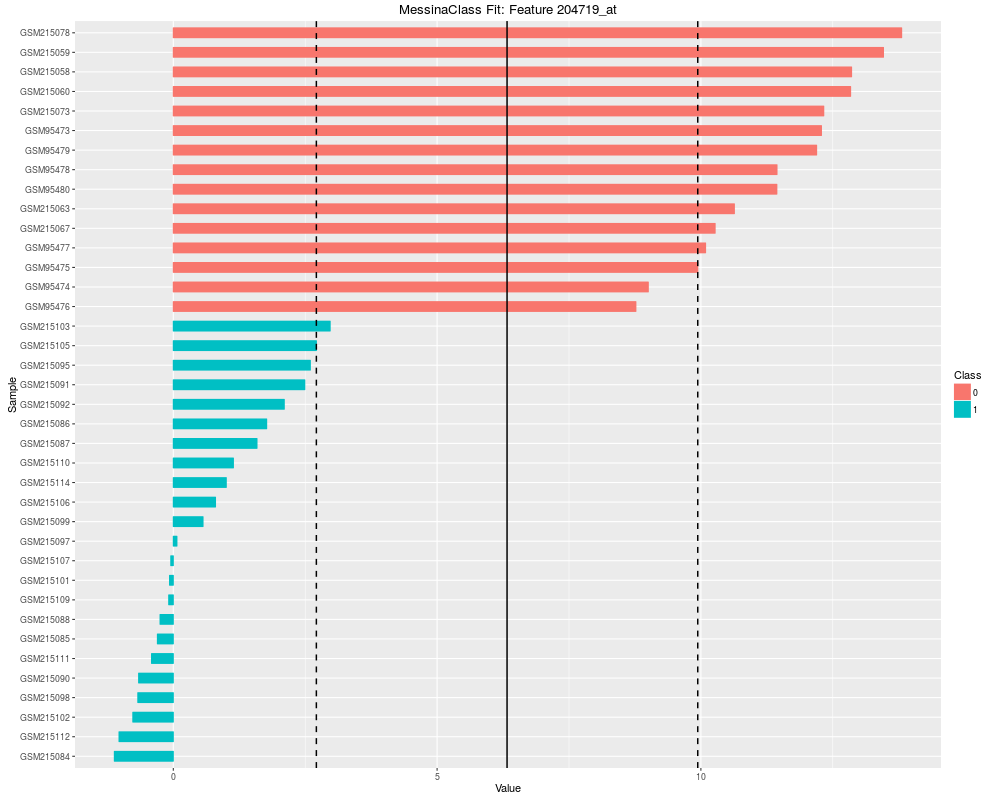
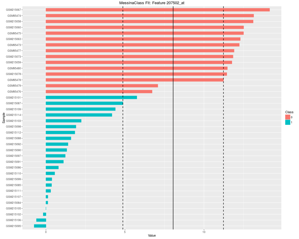
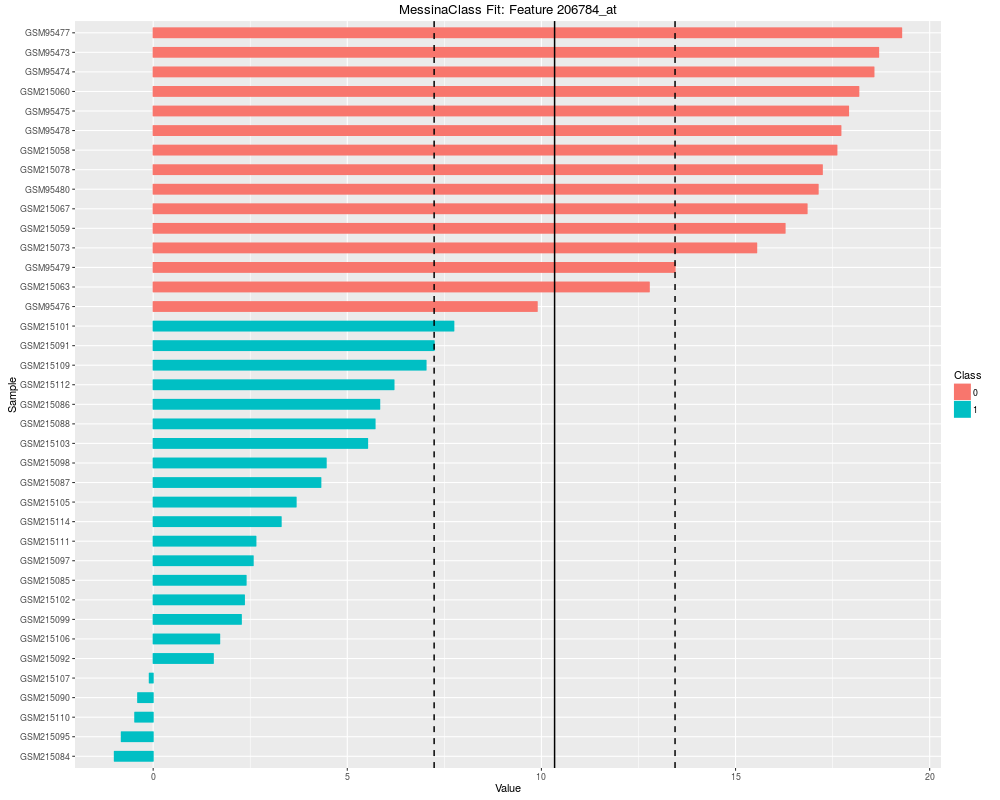
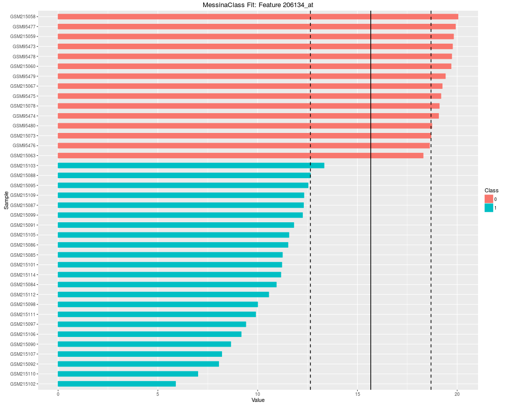
Plot the results of a Messina analysis on a classification / differential expression problem.

Description

Produces a separate plot for each supplied feature index (either as an index into the expression data x as-supplied, or as an index into the features sorted by Messina margin, depending on the value of sort_features), showing sample expression levels, group membership, threshold value, and margin locations. Two different types of plots can be produced. See the vignette for examples.

Usage

## S4 method for signature 'MessinaClassResult,missing'
plot(x, y, ...)

Arguments

x

the result of a Messina analysis, as returned by functions messina or messinaDE.

...

additional options to control the plot:

indices: a vector of indices of features to plot. If sort_features == FALSE, the indices are into the unsorted features, as originally supplied in x supplied to messina or messinaDE. If sort_features == TRUE, features are first sorted in order of decreasing margin, and then the indices in this parameter are plotted. For example, if indices == 2 and sort_features == FALSE, the second feature in x will be plotted. However, if sort_features == TRUE, the feature with the second best classifier margin will be plotted.
sort_features: a boolean indicating whether to sort features by decreasing margin size before selecting from indices. This affects the interpretation of the parameter 'indices'; for more details see the description of that parameter.
plot_type: a string giving the type of plot to produce, either "point" or "bar". "bar" is the default, and shows expression levels as horizontal bars. Although this representation is familiar, it can be misleading in the case of log-transformed data. In that case, the "point" plot type is preferable.

y

the y coordinates of points in the plot, optional if x is an appropriate structure.

Author(s)

Mark Pinese m.pinese@garvan.org.au

Examples

## Load some example data
library(antiProfilesData)
data(apColonData)

x = exprs(apColonData)
y = pData(apColonData)$SubType

## Subset the data to only tumour and normal samples
sel = y %in% c("normal", "tumor")
x = x[,sel]
y = y[sel]

## Run Messina to rank probesets on their classification ability, with
## classifiers needing to meet a minimum sensitivity of 0.95, and minimum
## specificity of 0.85.
fit = messina(x, y == "tumor", min_sens = 0.95, min_spec = 0.85)

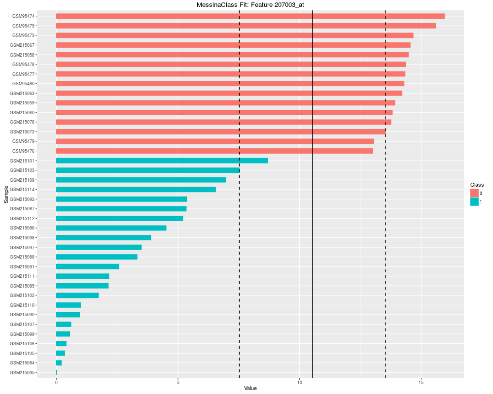
## Make bar plots of the five best fits
plot(fit, indices = 1:5, sort_features = TRUE, plot_type = "bar")

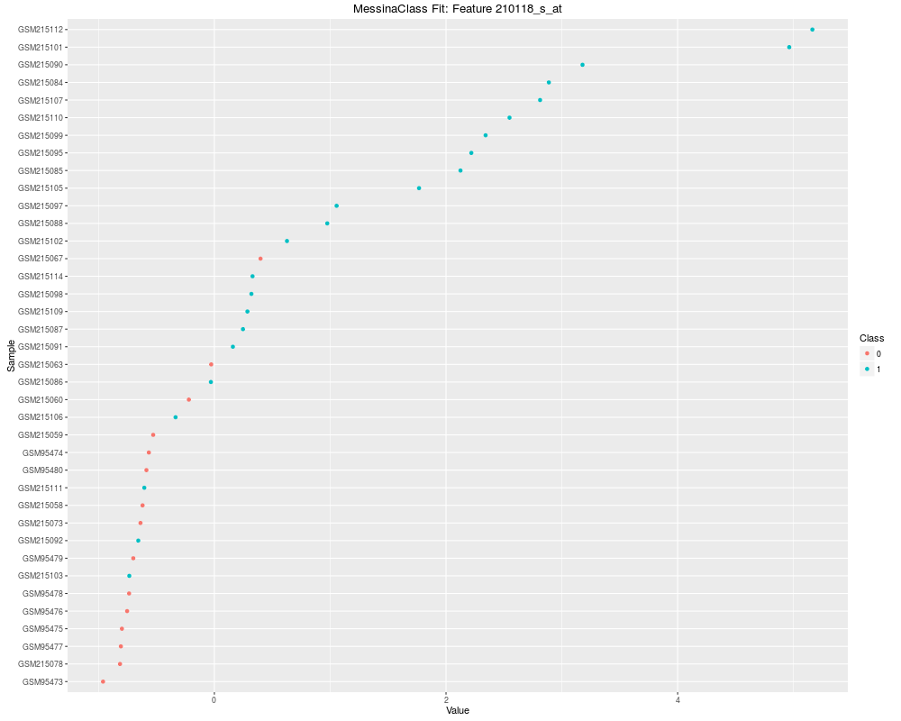
## Make a point plot of the fit to the 10th feature
plot(fit, indices = 10, sort_features = FALSE, plot_type = "point")

Results


R version 3.3.1 (2016-06-21) -- "Bug in Your Hair"
Copyright (C) 2016 The R Foundation for Statistical Computing
Platform: x86_64-pc-linux-gnu (64-bit)

R is free software and comes with ABSOLUTELY NO WARRANTY.
You are welcome to redistribute it under certain conditions.
Type 'license()' or 'licence()' for distribution details.

R is a collaborative project with many contributors.
Type 'contributors()' for more information and
'citation()' on how to cite R or R packages in publications.

Type 'demo()' for some demos, 'help()' for on-line help, or
'help.start()' for an HTML browser interface to help.
Type 'q()' to quit R.

> library(messina)
Loading required package: survival
> png(filename="/home/ddbj/snapshot/RGM3/R_BC/result/messina/plot-MessinaClassResult-missing-method.Rd_%03d_medium.png", width=480, height=480)
> ### Name: plot,MessinaClassResult,missing-method
> ### Title: Plot the results of a Messina analysis on a classification /
> ###   differential expression problem.
> ### Aliases: plot,MessinaClassResult,missing-method
> ###   plot,MessinaClassResult-method
> 
> ### ** Examples
> 
> ## Load some example data
> library(antiProfilesData)
Loading required package: Biobase
Loading required package: BiocGenerics
Loading required package: parallel

Attaching package: 'BiocGenerics'

The following objects are masked from 'package:parallel':

    clusterApply, clusterApplyLB, clusterCall, clusterEvalQ,
    clusterExport, clusterMap, parApply, parCapply, parLapply,
    parLapplyLB, parRapply, parSapply, parSapplyLB

The following objects are masked from 'package:stats':

    IQR, mad, xtabs

The following objects are masked from 'package:base':

    Filter, Find, Map, Position, Reduce, anyDuplicated, append,
    as.data.frame, cbind, colnames, do.call, duplicated, eval, evalq,
    get, grep, grepl, intersect, is.unsorted, lapply, lengths, mapply,
    match, mget, order, paste, pmax, pmax.int, pmin, pmin.int, rank,
    rbind, rownames, sapply, setdiff, sort, table, tapply, union,
    unique, unsplit

Welcome to Bioconductor

    Vignettes contain introductory material; view with
    'browseVignettes()'. To cite Bioconductor, see
    'citation("Biobase")', and for packages 'citation("pkgname")'.

> data(apColonData)
> 
> x = exprs(apColonData)
> y = pData(apColonData)$SubType
> 
> ## Subset the data to only tumour and normal samples
> sel = y %in% c("normal", "tumor")
> x = x[,sel]
> y = y[sel]
> 
> ## Run Messina to rank probesets on their classification ability, with
> ## classifiers needing to meet a minimum sensitivity of 0.95, and minimum
> ## specificity of 0.85.
> fit = messina(x, y == "tumor", min_sens = 0.95, min_spec = 0.85)
Performance bootstrapping...
  0% [                                                            ]   2% [=                                                           ]   4% [==                                                          ]   6% [===                                                         ]   8% [====                                                        ]   9% [=====                                                       ]  11% [======                                                      ]  13% [=======                                                     ]  15% [=========                                                   ]  17% [==========                                                  ]  19% [===========                                                 ]  21% [============                                                ]  22% [=============                                               ]  24% [==============                                              ]  26% [===============                                             ]  28% [================                                            ]  30% [=================                                           ]  32% [===================                                         ]  34% [====================                                        ]  36% [=====================                                       ]  37% [======================                                      ]  39% [=======================                                     ]  41% [========================                                    ]  43% [=========================                                   ]  45% [==========================                                  ]  47% [============================                                ]  49% [=============================                               ]  51% [==============================                              ]  52% [===============================                             ]  54% [================================                            ]  56% [=================================                           ]  58% [==================================                          ]  60% [===================================                         ]  62% [=====================================                       ]  64% [======================================                      ]  66% [=======================================                     ]  67% [========================================                    ]  69% [=========================================                   ]  71% [==========================================                  ]  73% [===========================================                 ]  75% [============================================                ]  77% [==============================================              ]  79% [===============================================             ]  81% [================================================            ]  82% [=================================================           ]  84% [==================================================          ]  86% [===================================================         ]  88% [====================================================        ]  90% [=====================================================       ]  92% [=======================================================     ]  94% [========================================================    ]  96% [=========================================================   ]  97% [==========================================================  ]  99% [=========================================================== ] 100% [============================================================] 
> 
> ## Make bar plots of the five best fits
> plot(fit, indices = 1:5, sort_features = TRUE, plot_type = "bar")
Warning messages:
1: Stacking not well defined when ymin != 0 
2: Stacking not well defined when ymin != 0 
3: Stacking not well defined when ymin != 0 
> 
> ## Make a point plot of the fit to the 10th feature
> plot(fit, indices = 10, sort_features = FALSE, plot_type = "point")
> 
> 
> 
> 
> 
> dev.off()
null device 
          1 
>