Generate a Basis Matrix for Natural Cubic Splines

Description

Generate the B-spline basis matrix for a natural cubic spline.

Usage

ns(x, df = NULL, knots = NULL, intercept = FALSE,
   Boundary.knots = range(x))

Arguments

Details

ns is based on the function spline.des. It generates a basis matrix for representing the family of piecewise-cubic splines with the specified sequence of interior knots, and the natural boundary conditions. These enforce the constraint that the function is linear beyond the boundary knots, which can either be supplied or default to the extremes of the data.

A primary use is in modeling formula to directly specify a natural spline term in a model: see the examples.

Value

A matrix of dimension length(x) * df where either df was supplied or if knots were supplied, df = length(knots) + 1 + intercept. Attributes are returned that correspond to the arguments to ns, and explicitly give the knots, Boundary.knots etc for use by predict.ns().

References

Hastie, T. J. (1992) Generalized additive models. Chapter 7 of Statistical Models in S eds J. M. Chambers and T. J. Hastie, Wadsworth & Brooks/Cole.

See Also

bs, predict.ns, SafePrediction

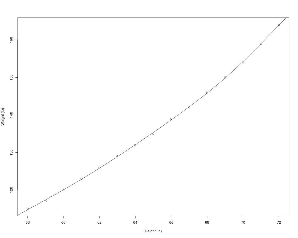
Examples

require(stats); require(graphics)
ns(women$height, df = 5)
summary(fm1 <- lm(weight ~ ns(height, df = 5), data = women))

## To see what knots were selected
attr(terms(fm1), "predvars")

## example of safe prediction
plot(women, xlab = "Height (in)", ylab = "Weight (lb)")
ht <- seq(57, 73, length.out = 200)
lines(ht, predict(fm1, data.frame(height = ht)))

Results

R version 3.3.1 (2016-06-21) -- "Bug in Your Hair"
Copyright (C) 2016 The R Foundation for Statistical Computing
Platform: x86_64-pc-linux-gnu (64-bit)

R is free software and comes with ABSOLUTELY NO WARRANTY.
You are welcome to redistribute it under certain conditions.
Type 'license()' or 'licence()' for distribution details.

R is a collaborative project with many contributors.
Type 'contributors()' for more information and
'citation()' on how to cite R or R packages in publications.

Type 'demo()' for some demos, 'help()' for on-line help, or
'help.start()' for an HTML browser interface to help.
Type 'q()' to quit R.

> library(splines)
> png(filename="/home/ddbj/snapshot/RGM3/R_rel/result/splines/ns.Rd_%03d_medium.png", width=480, height=480)
> ### Name: ns
> ### Title: Generate a Basis Matrix for Natural Cubic Splines
> ### Aliases: ns
> ### Keywords: smooth
> 
> ### ** Examples
> 
> require(stats); require(graphics)
> ns(women$height, df = 5)
                 1            2           3          4             5
 [1,] 0.000000e+00 0.000000e+00  0.00000000 0.00000000  0.0000000000
 [2,] 7.592323e-03 0.000000e+00 -0.08670223 0.26010669 -0.1734044626
 [3,] 6.073858e-02 0.000000e+00 -0.15030440 0.45091320 -0.3006088020
 [4,] 2.047498e-01 6.073858e-05 -0.16778345 0.50335034 -0.3355668952
 [5,] 4.334305e-01 1.311953e-02 -0.13244035 0.39732106 -0.2648807067
 [6,] 6.256681e-01 8.084305e-02 -0.07399720 0.22199159 -0.1479943948
 [7,] 6.477162e-01 2.468416e-01 -0.02616007 0.07993794 -0.0532919575
 [8,] 4.791667e-01 4.791667e-01  0.01406302 0.02031093 -0.0135406187
 [9,] 2.468416e-01 6.477162e-01  0.09733619 0.02286023 -0.0152401533
[10,] 8.084305e-02 6.256681e-01  0.27076826 0.06324188 -0.0405213106
[11,] 1.311953e-02 4.334305e-01  0.48059836 0.12526031 -0.0524087186
[12,] 6.073858e-05 2.047498e-01  0.59541597 0.19899261  0.0007809246
[13,] 0.000000e+00 6.073858e-02  0.50097182 0.27551020  0.1627793975
[14,] 0.000000e+00 7.592323e-03  0.22461127 0.35204082  0.4157555879
[15,] 0.000000e+00 0.000000e+00 -0.14285714 0.42857143  0.7142857143
attr(,"degree")
[1] 3
attr(,"knots")
 20%  40%  60%  80% 
60.8 63.6 66.4 69.2 
attr(,"Boundary.knots")
[1] 58 72
attr(,"intercept")
[1] FALSE
attr(,"class")
[1] "ns"     "basis"  "matrix"
> summary(fm1 <- lm(weight ~ ns(height, df = 5), data = women))

Call:
lm(formula = weight ~ ns(height, df = 5), data = women)

Residuals:
     Min       1Q   Median       3Q      Max 
-0.38333 -0.12585  0.07083  0.15401  0.30426 

Coefficients:
                    Estimate Std. Error t value Pr(>|t|)    
(Intercept)         114.7447     0.2338  490.88  < 2e-16 ***
ns(height, df = 5)1  15.9474     0.3699   43.12 9.69e-12 ***
ns(height, df = 5)2  25.1695     0.4323   58.23 6.55e-13 ***
ns(height, df = 5)3  33.2582     0.3541   93.93 8.91e-15 ***
ns(height, df = 5)4  50.7894     0.6062   83.78 2.49e-14 ***
ns(height, df = 5)5  45.0363     0.2784  161.75  < 2e-16 ***
---
Signif. codes:  0 '***' 0.001 '**' 0.01 '*' 0.05 '.' 0.1 ' ' 1

Residual standard error: 0.2645 on 9 degrees of freedom
Multiple R-squared:  0.9998,	Adjusted R-squared:  0.9997 
F-statistic:  9609 on 5 and 9 DF,  p-value: < 2.2e-16

> 
> ## To see what knots were selected
> attr(terms(fm1), "predvars")
list(weight, ns(height, knots = c(60.8, 63.6, 66.4, 69.2), Boundary.knots = c(58, 
72), intercept = FALSE))
> 
> ## example of safe prediction
> plot(women, xlab = "Height (in)", ylab = "Weight (lb)")
> ht <- seq(57, 73, length.out = 200)
> lines(ht, predict(fm1, data.frame(height = ht)))
> ## Don't show: 
> ## Consistency:
> x <- c(1:3, 5:6)
> stopifnot(identical(ns(x), ns(x, df = 1)),
+           identical(ns(x, df = 2), ns(x, df = 2, knots = NULL)), # not true till 2.15.2
+           !is.null(kk <- attr(ns(x), "knots")), # not true till 1.5.1
+           length(kk) == 0)
> ## End(Don't show)
> 
> 
> 
> 
> 
> dev.off()
null device 
          1 
>