Supported by Dr. Osamu Ogasawara and  . . |
|
Last data update: 2014.03.03 |
Compute Tukey Honest Significant DifferencesDescriptionCreate a set of confidence intervals on the differences between the means of the levels of a factor with the specified family-wise probability of coverage. The intervals are based on the Studentized range statistic, Tukey's ‘Honest Significant Difference’ method. UsageTukeyHSD(x, which, ordered = FALSE, conf.level = 0.95, ...) Arguments
DetailsThis is a generic function: the description here applies to the method
for fits of class When comparing the means for the levels of a factor in an analysis of variance, a simple comparison using t-tests will inflate the probability of declaring a significant difference when it is not in fact present. This because the intervals are calculated with a given coverage probability for each interval but the interpretation of the coverage is usually with respect to the entire family of intervals. John Tukey introduced intervals based on the range of the sample means rather than the individual differences. The intervals returned by this function are based on this Studentized range statistics. The intervals constructed in this way would only apply exactly to balanced designs where there are the same number of observations made at each level of the factor. This function incorporates an adjustment for sample size that produces sensible intervals for mildly unbalanced designs. If ValueA list of class There are Author(s)Douglas Bates ReferencesMiller, R. G. (1981) Simultaneous Statistical Inference. Springer. Yandell, B. S. (1997) Practical Data Analysis for Designed Experiments. Chapman & Hall. See Also
Examplesrequire(graphics) summary(fm1 <- aov(breaks ~ wool + tension, data = warpbreaks)) TukeyHSD(fm1, "tension", ordered = TRUE) plot(TukeyHSD(fm1, "tension")) Results
R version 3.3.1 (2016-06-21) -- "Bug in Your Hair"
Copyright (C) 2016 The R Foundation for Statistical Computing
Platform: x86_64-pc-linux-gnu (64-bit)
R is free software and comes with ABSOLUTELY NO WARRANTY.
You are welcome to redistribute it under certain conditions.
Type 'license()' or 'licence()' for distribution details.
R is a collaborative project with many contributors.
Type 'contributors()' for more information and
'citation()' on how to cite R or R packages in publications.
Type 'demo()' for some demos, 'help()' for on-line help, or
'help.start()' for an HTML browser interface to help.
Type 'q()' to quit R.
> library(stats)
> png(filename="/home/ddbj/snapshot/RGM3/R_rel/result/stats/TukeyHSD.Rd_%03d_medium.png", width=480, height=480)
> ### Name: TukeyHSD
> ### Title: Compute Tukey Honest Significant Differences
> ### Aliases: TukeyHSD
> ### Keywords: models design
>
> ### ** Examples
>
> require(graphics)
>
> summary(fm1 <- aov(breaks ~ wool + tension, data = warpbreaks))
Df Sum Sq Mean Sq F value Pr(>F)
wool 1 451 450.7 3.339 0.07361 .
tension 2 2034 1017.1 7.537 0.00138 **
Residuals 50 6748 135.0
---
Signif. codes: 0 '***' 0.001 '**' 0.01 '*' 0.05 '.' 0.1 ' ' 1
> TukeyHSD(fm1, "tension", ordered = TRUE)
Tukey multiple comparisons of means
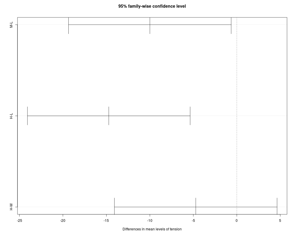
95% family-wise confidence level
factor levels have been ordered
Fit: aov(formula = breaks ~ wool + tension, data = warpbreaks)
$tension
diff lwr upr p adj
M-H 4.722222 -4.6311985 14.07564 0.4474210
L-H 14.722222 5.3688015 24.07564 0.0011218
L-M 10.000000 0.6465793 19.35342 0.0336262
> plot(TukeyHSD(fm1, "tension"))
>
>
>
>
>
> dev.off()
null device
1
>
|