Empirical Cumulative Distribution Function

Description

Compute an empirical cumulative distribution function, with several methods for plotting, printing and computing with such an “ecdf” object.

Usage

ecdf(x)

## S3 method for class 'ecdf'
plot(x, ..., ylab="Fn(x)", verticals = FALSE,
     col.01line = "gray70", pch = 19)

## S3 method for class 'ecdf'
print(x, digits= getOption("digits") - 2, ...)

## S3 method for class 'ecdf'
summary(object, ...)
## S3 method for class 'ecdf'
quantile(x, ...)

Arguments

Details

The e.c.d.f. (empirical cumulative distribution function) Fn is a step function with jumps i/n at observation values, where i is the number of tied observations at that value. Missing values are ignored.

For observations x= (x1,x2, ... xn), Fn is the fraction of observations less or equal to t, i.e.,

Fn(t) = #{xi <= t}/n = 1/n sum(i=1,n) Indicator(xi <= t).

The function plot.ecdf which implements the plot method for ecdf objects, is implemented via a call to plot.stepfun; see its documentation.

Value

For ecdf, a function of class "ecdf", inheriting from the "stepfun" class, and hence inheriting a knots() method.

For the summary method, a summary of the knots of object with a "header" attribute.

The quantile(obj, ...) method computes the same quantiles as quantile(x, ...) would where x is the original sample.

Note

The objects of class "ecdf" are not intended to be used for permanent storage and may change structure between versions of R (and did at R 3.0.0). They can usually be re-created by

    eval(attr(old_obj, "call"), environment(old_obj))

since the data used is stored as part of the object's environment.

Author(s)

Martin Maechler; fixes and new features by other R-core members.

See Also

stepfun, the more general class of step functions, approxfun and splinefun.

Examples

##-- Simple didactical  ecdf  example :
x <- rnorm(12)
Fn <- ecdf(x)
Fn     # a *function*
Fn(x)  # returns the percentiles for x
tt <- seq(-2, 2, by = 0.1)
12 * Fn(tt) # Fn is a 'simple' function {with values k/12}
summary(Fn)
##--> see below for graphics
knots(Fn)  # the unique data values {12 of them if there were no ties}

y <- round(rnorm(12), 1); y[3] <- y[1]
Fn12 <- ecdf(y)
Fn12
knots(Fn12) # unique values (always less than 12!)
summary(Fn12)
summary.stepfun(Fn12)

## Advanced: What's inside the function closure?
ls(environment(Fn12))
##[1] "f"  "method"  "n"  "x"  "y"  "yleft"  "yright"
utils::ls.str(environment(Fn12))
stopifnot(all.equal(quantile(Fn12), quantile(y)))

###----------------- Plotting --------------------------
require(graphics)

op <- par(mfrow = c(3, 1), mgp = c(1.5, 0.8, 0), mar =  .1+c(3,3,2,1))

F10 <- ecdf(rnorm(10))
summary(F10)

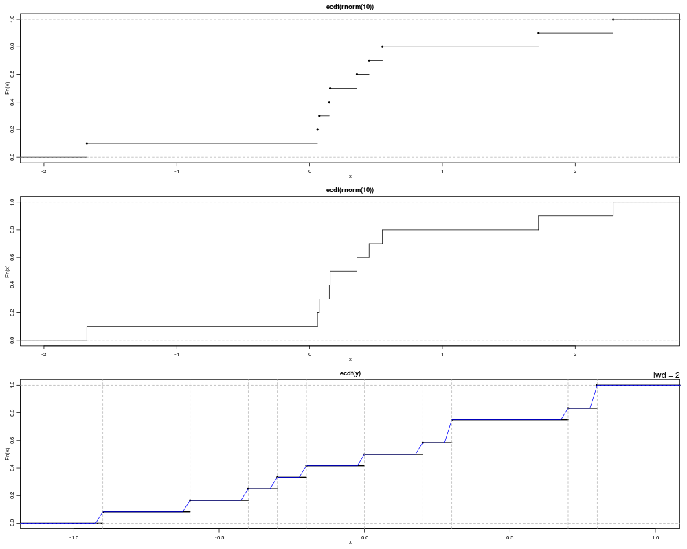
plot(F10)
plot(F10, verticals = TRUE, do.points = FALSE)

plot(Fn12 , lwd = 2) ; mtext("lwd = 2", adj = 1)
xx <- unique(sort(c(seq(-3, 2, length = 201), knots(Fn12))))
lines(xx, Fn12(xx), col = "blue")
abline(v = knots(Fn12), lty = 2, col = "gray70")

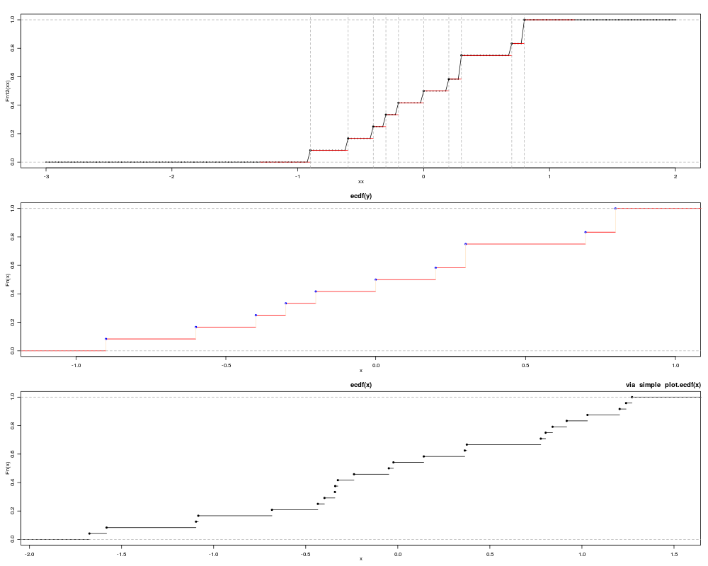
plot(xx, Fn12(xx), type = "o", cex = .1)  #- plot.default {ugly}
plot(Fn12, col.hor = "red", add =  TRUE)  #- plot method
abline(v = knots(Fn12), lty = 2, col = "gray70")
## luxury plot
plot(Fn12, verticals = TRUE, col.points = "blue",
     col.hor = "red", col.vert = "bisque")

##-- this works too (automatic call to  ecdf(.)):
plot.ecdf(rnorm(24))
title("via  simple  plot.ecdf(x)", adj = 1)

par(op)

Results

R version 3.3.1 (2016-06-21) -- "Bug in Your Hair"
Copyright (C) 2016 The R Foundation for Statistical Computing
Platform: x86_64-pc-linux-gnu (64-bit)

R is free software and comes with ABSOLUTELY NO WARRANTY.
You are welcome to redistribute it under certain conditions.
Type 'license()' or 'licence()' for distribution details.

R is a collaborative project with many contributors.
Type 'contributors()' for more information and
'citation()' on how to cite R or R packages in publications.

Type 'demo()' for some demos, 'help()' for on-line help, or
'help.start()' for an HTML browser interface to help.
Type 'q()' to quit R.

> library(stats)
> png(filename="/home/ddbj/snapshot/RGM3/R_rel/result/stats/ecdf.Rd_%03d_medium.png", width=480, height=480)
> ### Name: ecdf
> ### Title: Empirical Cumulative Distribution Function
> ### Aliases: ecdf plot.ecdf print.ecdf summary.ecdf quantile.ecdf
> ### Keywords: dplot hplot
> 
> ### ** Examples
> 
> ##-- Simple didactical  ecdf  example :
> x <- rnorm(12)
> Fn <- ecdf(x)
> Fn     # a *function*
Empirical CDF 
Call: ecdf(x)
 x[1:12] = -1.8543, -1.0317, -0.50268,  ..., 0.95994, 1.5052
> Fn(x)  # returns the percentiles for x
 [1] 0.41666667 0.75000000 0.25000000 0.91666667 1.00000000 0.83333333
 [7] 0.08333333 0.58333333 0.50000000 0.66666667 0.33333333 0.16666667
> tt <- seq(-2, 2, by = 0.1)
> 12 * Fn(tt) # Fn is a 'simple' function {with values k/12}
 [1]  0  0  1  1  1  1  1  1  1  1  2  2  2  2  2  3  4  4  6  7  7  7  7  7  8
[26]  9  9  9 10 10 11 11 11 11 11 11 12 12 12 12 12
> summary(Fn)
Empirical CDF:	  12 unique values with summary
    Min.  1st Qu.   Median     Mean  3rd Qu.     Max. 
-1.85400 -0.50040 -0.20790 -0.04521  0.55160  1.50500 
> ##--> see below for graphics
> knots(Fn)  # the unique data values {12 of them if there were no ties}
 [1] -1.8542947 -1.0317204 -0.5026786 -0.4996172 -0.2450411 -0.2193635
 [7] -0.1963682  0.3171520  0.4911416  0.7331731  0.9599411  1.5051665
> 
> y <- round(rnorm(12), 1); y[3] <- y[1]
> Fn12 <- ecdf(y)
> Fn12
Empirical CDF 
Call: ecdf(y)
 x[1:11] =   -2.3,   -1.3,   -1.2,  ...,    0.5,    1.1
> knots(Fn12) # unique values (always less than 12!)
 [1] -2.3 -1.3 -1.2 -1.1 -1.0 -0.9 -0.7 -0.5  0.1  0.5  1.1
> summary(Fn12)
Empirical CDF:	  11 unique values with summary
   Min. 1st Qu.  Median    Mean 3rd Qu.    Max. 
-2.3000 -1.1500 -0.9000 -0.6636 -0.2000  1.1000 
> summary.stepfun(Fn12)
Step function with continuity 'f'= 0 ,  11 knots with summary
   Min. 1st Qu.  Median    Mean 3rd Qu.    Max. 
-2.3000 -1.1500 -0.9000 -0.6636 -0.2000  1.1000 

and	12 plateau levels (y) with summary
   Min. 1st Qu.  Median    Mean 3rd Qu.    Max. 
 0.0000  0.2292  0.4583  0.4931  0.7708  1.0000 
> 
> ## Advanced: What's inside the function closure?
> ls(environment(Fn12))
[1] "f"      "method" "nobs"   "x"      "y"      "yleft"  "yright"
> ##[1] "f"  "method"  "n"  "x"  "y"  "yleft"  "yright"
> utils::ls.str(environment(Fn12))
f :  num 0
method :  int 2
nobs :  int 12
x :  num [1:11] -2.3 -1.3 -1.2 -1.1 -1 -0.9 -0.7 -0.5 0.1 0.5 ...
y :  num [1:11] 0.0833 0.1667 0.25 0.3333 0.4167 ...
yleft :  num 0
yright :  num 1
> stopifnot(all.equal(quantile(Fn12), quantile(y)))
> 
> ###----------------- Plotting --------------------------
> require(graphics)
> 
> op <- par(mfrow = c(3, 1), mgp = c(1.5, 0.8, 0), mar =  .1+c(3,3,2,1))
> 
> F10 <- ecdf(rnorm(10))
> summary(F10)
Empirical CDF:	  10 unique values with summary
   Min. 1st Qu.  Median    Mean 3rd Qu.    Max. 
-1.4110 -0.7928  0.4420  0.1845  0.9632  1.7300 
> 
> plot(F10)
> plot(F10, verticals = TRUE, do.points = FALSE)
> 
> plot(Fn12 , lwd = 2) ; mtext("lwd = 2", adj = 1)
> xx <- unique(sort(c(seq(-3, 2, length = 201), knots(Fn12))))
> lines(xx, Fn12(xx), col = "blue")
> abline(v = knots(Fn12), lty = 2, col = "gray70")
> 
> plot(xx, Fn12(xx), type = "o", cex = .1)  #- plot.default {ugly}
> plot(Fn12, col.hor = "red", add =  TRUE)  #- plot method
> abline(v = knots(Fn12), lty = 2, col = "gray70")
> ## luxury plot
> plot(Fn12, verticals = TRUE, col.points = "blue",
+      col.hor = "red", col.vert = "bisque")
> 
> ##-- this works too (automatic call to  ecdf(.)):
> plot.ecdf(rnorm(24))
> title("via  simple  plot.ecdf(x)", adj = 1)
> 
> par(op)
> 
> 
> 
> 
> 
> dev.off()
null device 
          1 
>