Supported by Dr. Osamu Ogasawara and  . . |
|
Last data update: 2014.03.03 |
Two-way Interaction PlotDescriptionPlots the mean (or other summary) of the response for two-way combinations of factors, thereby illustrating possible interactions. Usage
interaction.plot(x.factor, trace.factor, response, fun = mean,
                 type = c("l", "p", "b", "o", "c"), legend = TRUE,
                 trace.label = deparse(substitute(trace.factor)),
                 fixed = FALSE,
                 xlab = deparse(substitute(x.factor)),
                 ylab = ylabel,
                 ylim = range(cells, na.rm = TRUE),
                 lty = nc:1, col = 1, pch = c(1:9, 0, letters),
                 xpd = NULL, leg.bg = par("bg"), leg.bty = "n",
                 xtick = FALSE, xaxt = par("xaxt"), axes = TRUE,
                 ...)
Arguments
DetailsBy default the levels of The response and hence its summary can contain missing values. If so, the missing values and the line segments joining them are omitted from the plot (and this can be somewhat disconcerting). The graphics parameters NoteSome of the argument names and the precise behaviour are chosen for S-compatibility. ReferencesChambers, J. M., Freeny, A and Heiberger, R. M. (1992) Analysis of variance; designed experiments. Chapter 5 of Statistical Models in S eds J. M. Chambers and T. J. Hastie, Wadsworth & Brooks/Cole. Examples
require(graphics)
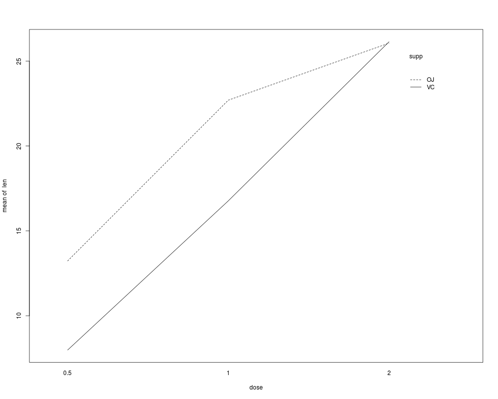
with(ToothGrowth, {
interaction.plot(dose, supp, len, fixed = TRUE)
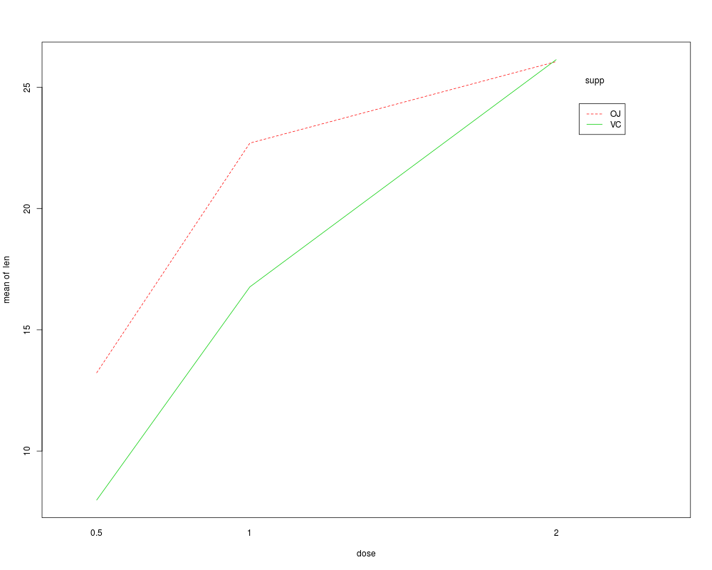
dose <- ordered(dose)
interaction.plot(dose, supp, len, fixed = TRUE, col = 2:3, leg.bty = "o")
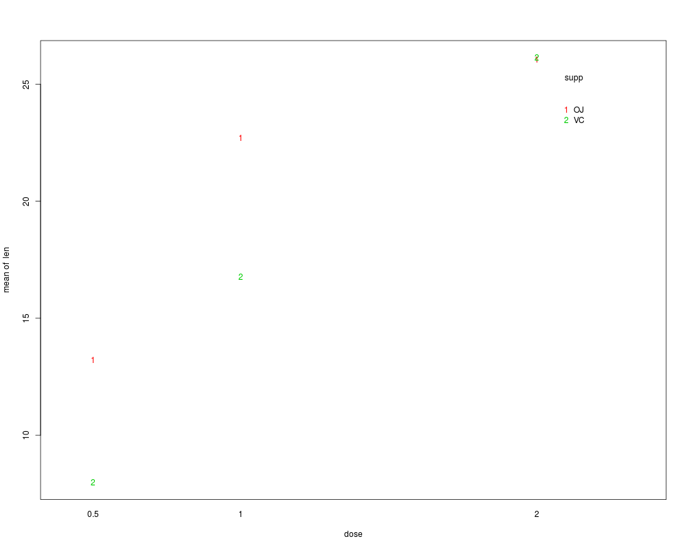
interaction.plot(dose, supp, len, fixed = TRUE, col = 2:3, type = "p")
})
with(OrchardSprays, {
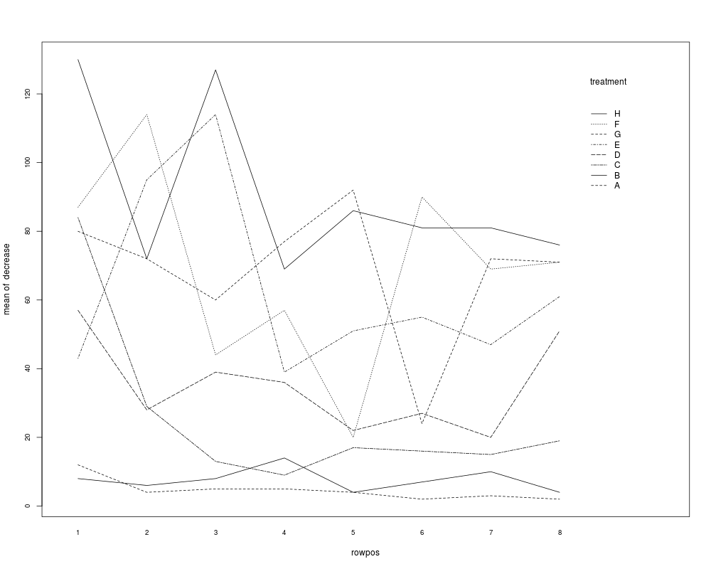
interaction.plot(treatment, rowpos, decrease)
interaction.plot(rowpos, treatment, decrease, cex.axis = 0.8)
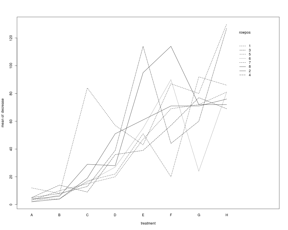
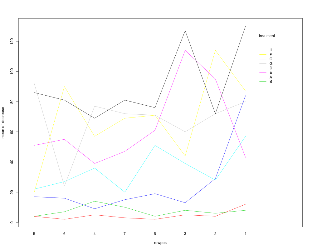
## order the rows by their mean effect
rowpos <- factor(rowpos,
levels = sort.list(tapply(decrease, rowpos, mean)))
interaction.plot(rowpos, treatment, decrease, col = 2:9, lty = 1)
})
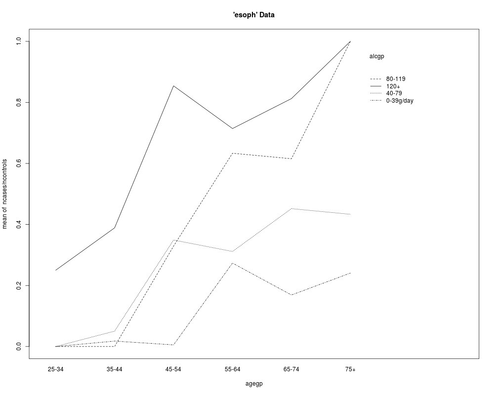
with(esoph, {
interaction.plot(agegp, alcgp, ncases/ncontrols, main = "'esoph' Data")
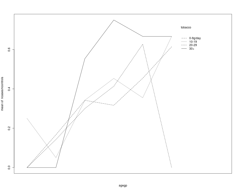
interaction.plot(agegp, tobgp, ncases/ncontrols, trace.label = "tobacco",
fixed = TRUE, xaxt = "n")
})
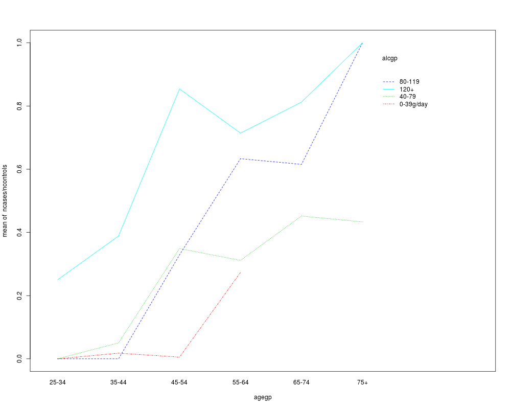
## deal with NAs:
esoph[66,] # second to last age group: 65-74
esophNA <- esoph; esophNA$ncases[66] <- NA
with(esophNA, {
interaction.plot(agegp, alcgp, ncases/ncontrols, col = 2:5)
# doesn't show *last* group either
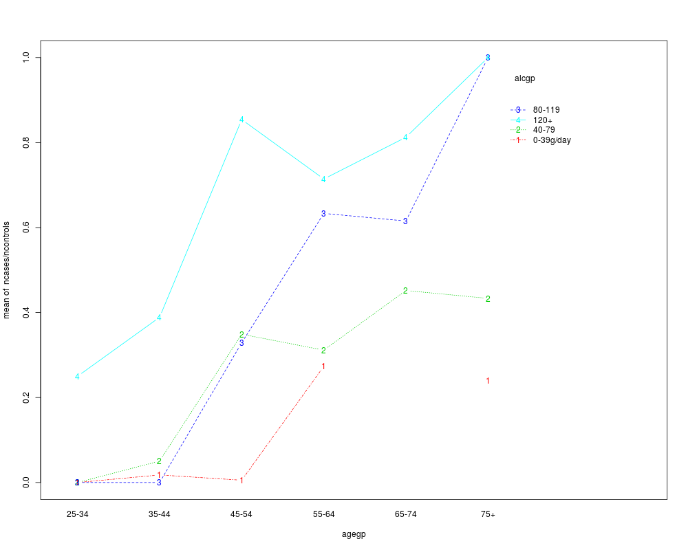
interaction.plot(agegp, alcgp, ncases/ncontrols, col = 2:5, type = "b")
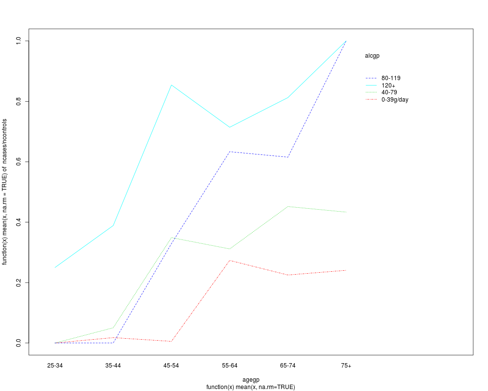
## alternative take non-NA's {"cheating"}
interaction.plot(agegp, alcgp, ncases/ncontrols, col = 2:5,
fun = function(x) mean(x, na.rm = TRUE),
sub = "function(x) mean(x, na.rm=TRUE)")
})
rm(esophNA) # to clear up
Results
R version 3.3.1 (2016-06-21) -- "Bug in Your Hair"
Copyright (C) 2016 The R Foundation for Statistical Computing
Platform: x86_64-pc-linux-gnu (64-bit)

R is free software and comes with ABSOLUTELY NO WARRANTY.
You are welcome to redistribute it under certain conditions.
Type 'license()' or 'licence()' for distribution details.

R is a collaborative project with many contributors.
Type 'contributors()' for more information and
'citation()' on how to cite R or R packages in publications.

Type 'demo()' for some demos, 'help()' for on-line help, or
'help.start()' for an HTML browser interface to help.
Type 'q()' to quit R.

> library(stats)
> png(filename="/home/ddbj/snapshot/RGM3/R_rel/result/stats/interaction.plot.Rd_%03d_medium.png", width=480, height=480)
> ### Name: interaction.plot
> ### Title: Two-way Interaction Plot
> ### Aliases: interaction.plot
> ### Keywords: hplot
>
> ### ** Examples
>
> require(graphics)
>
> with(ToothGrowth, {
+ interaction.plot(dose, supp, len, fixed = TRUE)
+ dose <- ordered(dose)
+ interaction.plot(dose, supp, len, fixed = TRUE, col = 2:3, leg.bty = "o")
+ interaction.plot(dose, supp, len, fixed = TRUE, col = 2:3, type = "p")
+ })
>
> with(OrchardSprays, {
+   interaction.plot(treatment, rowpos, decrease)
+   interaction.plot(rowpos, treatment, decrease, cex.axis = 0.8)
+   ## order the rows by their mean effect
+   rowpos <- factor(rowpos,
+                    levels = sort.list(tapply(decrease, rowpos, mean)))
+   interaction.plot(rowpos, treatment, decrease, col = 2:9, lty = 1)
+ })
>
> with(esoph, {
+   interaction.plot(agegp, alcgp, ncases/ncontrols, main = "'esoph' Data")
+   interaction.plot(agegp, tobgp, ncases/ncontrols, trace.label = "tobacco",
+                    fixed = TRUE, xaxt = "n")
+ })
> ## deal with NAs:
> esoph[66,] # second to last age group: 65-74
   agegp     alcgp tobgp ncases ncontrols
66 65-74 0-39g/day   30+      0         2
> esophNA <- esoph; esophNA$ncases[66] <- NA
> with(esophNA, {
+   interaction.plot(agegp, alcgp, ncases/ncontrols, col = 2:5)
+                                 # doesn't show *last* group either
+   interaction.plot(agegp, alcgp, ncases/ncontrols, col = 2:5, type = "b")
+   ## alternative take non-NA's  {"cheating"}
+   interaction.plot(agegp, alcgp, ncases/ncontrols, col = 2:5,
+                    fun = function(x) mean(x, na.rm = TRUE),
+                    sub = "function(x) mean(x, na.rm=TRUE)")
+ })
> rm(esophNA) # to clear up
>
>
>
>
>
> dev.off()
null device
          1
>
|