Accessing Linear Model Fits

Description

All these functions are methods for class "lm" objects.

Usage

## S3 method for class 'lm'
family(object, ...)

## S3 method for class 'lm'
formula(x, ...)

## S3 method for class 'lm'
residuals(object,
          type = c("working", "response", "deviance", "pearson",
                   "partial"),
          ...)

## S3 method for class 'lm'
labels(object, ...)

Arguments

Details

The generic accessor functions coef, effects, fitted and residuals can be used to extract various useful features of the value returned by lm.

The working and response residuals are ‘observed - fitted’. The deviance and pearson residuals are weighted residuals, scaled by the square root of the weights used in fitting. The partial residuals are a matrix with each column formed by omitting a term from the model. In all these, zero weight cases are never omitted (as opposed to the standardized rstudent residuals, and the weighted.residuals).

How residuals treats cases with missing values in the original fit is determined by the na.action argument of that fit. If na.action = na.omit omitted cases will not appear in the residuals, whereas if na.action = na.exclude they will appear, with residual value NA. See also naresid.

The "lm" method for generic labels returns the term labels for estimable terms, that is the names of the terms with an least one estimable coefficient.

References

Chambers, J. M. (1992) Linear models. Chapter 4 of Statistical Models in S eds J. M. Chambers and T. J. Hastie, Wadsworth & Brooks/Cole.

See Also

The model fitting function lm, anova.lm.

coef, deviance, df.residual, effects, fitted, glm for generalized linear models, influence (etc on that page) for regression diagnostics, weighted.residuals, residuals, residuals.glm, summary.lm, weights.

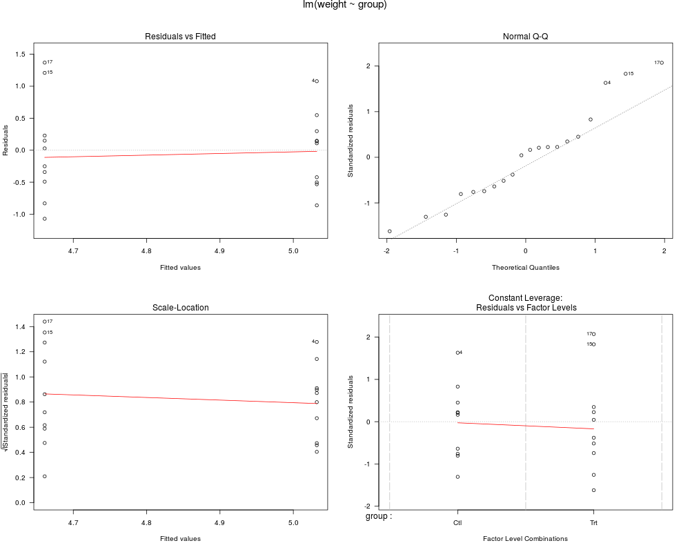
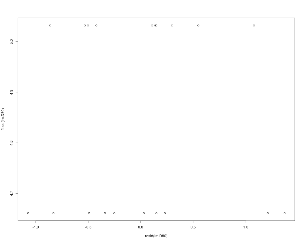
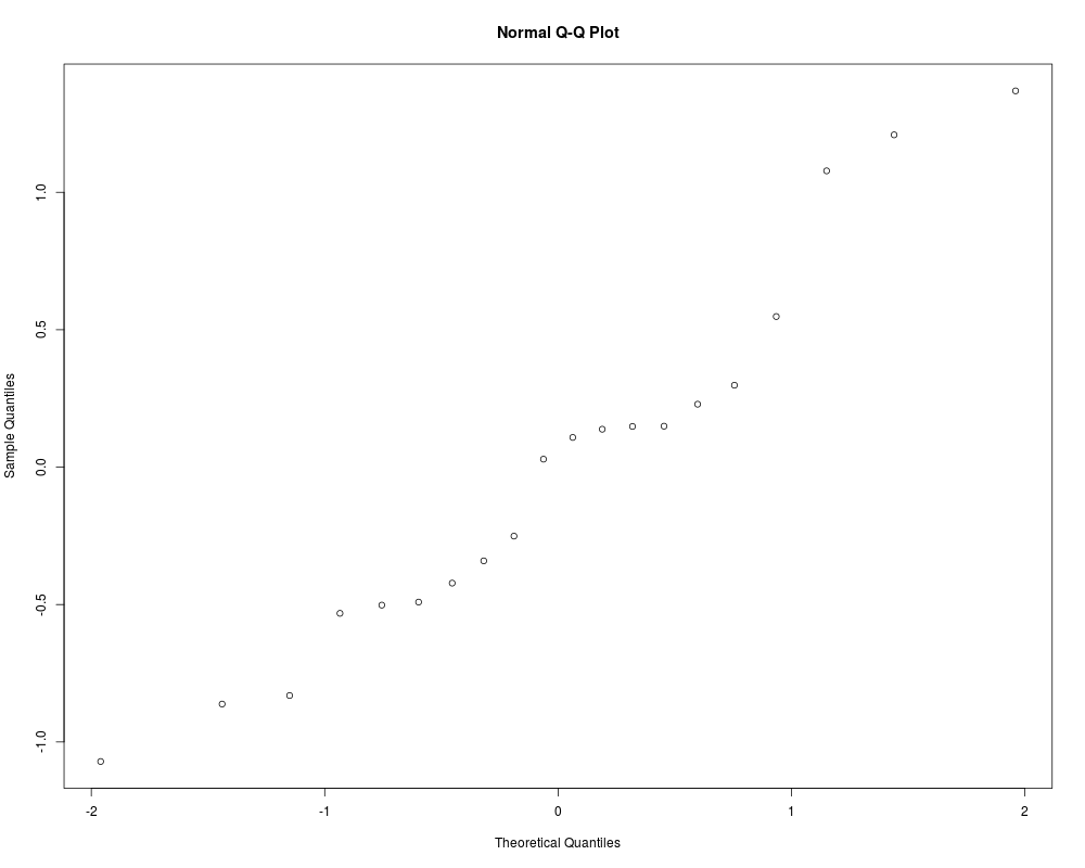
influence.measures for deletion diagnostics, including standardized (rstandard) and studentized (rstudent) residuals.

Examples

##-- Continuing the  lm(.) example:
coef(lm.D90) # the bare coefficients

## The 2 basic regression diagnostic plots [plot.lm(.) is preferred]
plot(resid(lm.D90), fitted(lm.D90)) # Tukey-Anscombe's
abline(h = 0, lty = 2, col = "gray")

qqnorm(residuals(lm.D90))

Results

R version 3.3.1 (2016-06-21) -- "Bug in Your Hair"
Copyright (C) 2016 The R Foundation for Statistical Computing
Platform: x86_64-pc-linux-gnu (64-bit)

R is free software and comes with ABSOLUTELY NO WARRANTY.
You are welcome to redistribute it under certain conditions.
Type 'license()' or 'licence()' for distribution details.

R is a collaborative project with many contributors.
Type 'contributors()' for more information and
'citation()' on how to cite R or R packages in publications.

Type 'demo()' for some demos, 'help()' for on-line help, or
'help.start()' for an HTML browser interface to help.
Type 'q()' to quit R.

> library(stats)
> png(filename="/home/ddbj/snapshot/RGM3/R_rel/result/stats/lm.summaries.Rd_%03d_medium.png", width=480, height=480)
> ### Name: lm.summaries
> ### Title: Accessing Linear Model Fits
> ### Aliases: family.lm formula.lm residuals.lm labels.lm
> ### Keywords: regression models
> 
> ### ** Examples
> 
> ## Don't show: 
> utils::example("lm", echo = FALSE)
> ## End(Don't show)
> ##-- Continuing the  lm(.) example:
> coef(lm.D90) # the bare coefficients
groupCtl groupTrt 
   5.032    4.661 
> 
> ## The 2 basic regression diagnostic plots [plot.lm(.) is preferred]
> plot(resid(lm.D90), fitted(lm.D90)) # Tukey-Anscombe's
> abline(h = 0, lty = 2, col = "gray")
> 
> qqnorm(residuals(lm.D90))
> 
> 
> 
> 
> 
> dev.off()
null device 
          1 
>