Supported by Dr. Osamu Ogasawara and  . . |
|
Last data update: 2014.03.03 |
One Dimensional OptimizationDescriptionThe function
Usage
optimize(f, interval, ..., lower = min(interval), upper = max(interval),
         maximum = FALSE,
         tol = .Machine$double.eps^0.25)
optimise(f, interval, ..., lower = min(interval), upper = max(interval),
         maximum = FALSE,
         tol = .Machine$double.eps^0.25)
Arguments
DetailsNote that arguments after The method used is a combination of golden section search and
successive parabolic interpolation, and was designed for use with
continuous functions. Convergence is never much slower
than that for a Fibonacci search. If The function The first evaluation of
The argument passed to ValueA list with components SourceA C translation of Fortran code http://www.netlib.org/fmm/fmin.f
(author(s) unstated)
based on the Algol 60 procedure ReferencesBrent, R. (1973) Algorithms for Minimization without Derivatives. Englewood Cliffs N.J.: Prentice-Hall. See Also
Examples
require(graphics)
f <- function (x, a) (x - a)^2
xmin <- optimize(f, c(0, 1), tol = 0.0001, a = 1/3)
xmin
## See where the function is evaluated:
optimize(function(x) x^2*(print(x)-1), lower = 0, upper = 10)
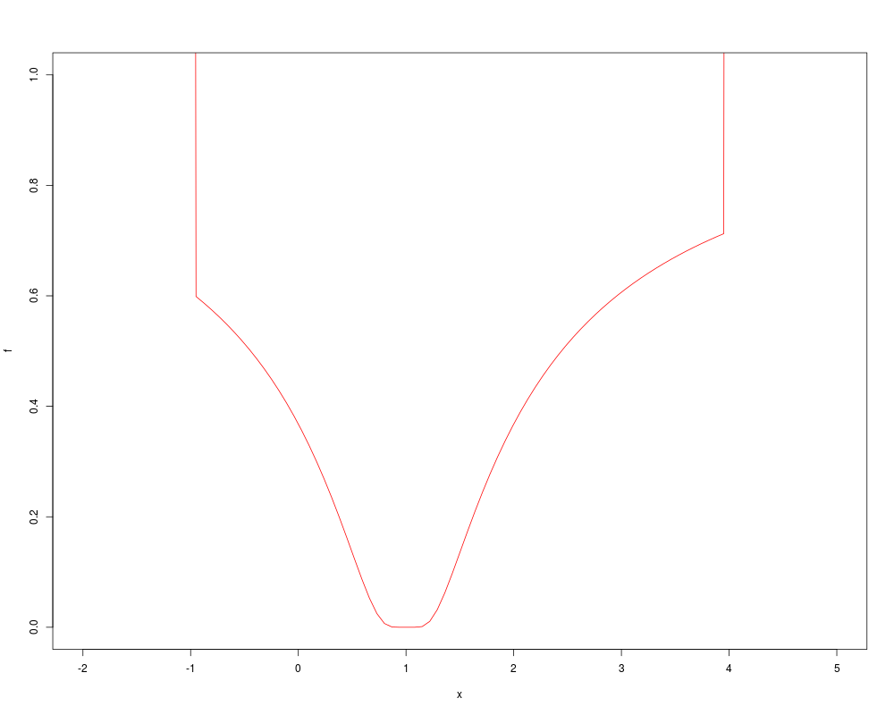
## "wrong" solution with unlucky interval and piecewise constant f():
f <- function(x) ifelse(x > -1, ifelse(x < 4, exp(-1/abs(x - 1)), 10), 10)
fp <- function(x) { print(x); f(x) }
plot(f, -2,5, ylim = 0:1, col = 2)
optimize(fp, c(-4, 20)) # doesn't see the minimum
optimize(fp, c(-7, 20)) # ok
Results
R version 3.3.1 (2016-06-21) -- "Bug in Your Hair"
Copyright (C) 2016 The R Foundation for Statistical Computing
Platform: x86_64-pc-linux-gnu (64-bit)

R is free software and comes with ABSOLUTELY NO WARRANTY.
You are welcome to redistribute it under certain conditions.
Type 'license()' or 'licence()' for distribution details.

R is a collaborative project with many contributors.
Type 'contributors()' for more information and
'citation()' on how to cite R or R packages in publications.

Type 'demo()' for some demos, 'help()' for on-line help, or
'help.start()' for an HTML browser interface to help.
Type 'q()' to quit R.

> library(stats)
> png(filename="/home/ddbj/snapshot/RGM3/R_rel/result/stats/optimize.Rd_%03d_medium.png", width=480, height=480)
> ### Name: optimize
> ### Title: One Dimensional Optimization
> ### Aliases: optimize optimise
> ### Keywords: optimize
>
> ### ** Examples
>
> require(graphics)
>
> f <- function (x, a) (x - a)^2
> xmin <- optimize(f, c(0, 1), tol = 0.0001, a = 1/3)
> xmin
$minimum
[1] 0.3333333

$objective
[1] 0

>
> ## See where the function is evaluated:
> optimize(function(x) x^2*(print(x)-1), lower = 0, upper = 10)
[1] 3.81966
[1] 6.18034
[1] 2.36068
[1] 2.077939
[1] 1.505823
[1] 0.9306496
[1] 0.9196752
[1] 0.772905
[1] 0.4776816
[1] 0.6491436
[1] 0.656315
[1] 0.6653777
[1] 0.6667786
[1] 0.6666728
[1] 0.6666321
[1] 0.6667135
[1] 0.6666728
$minimum
[1] 0.6666728

$objective
[1] -0.1481481

>
> ## "wrong" solution with unlucky interval and piecewise constant f():
> f  <- function(x) ifelse(x > -1, ifelse(x < 4, exp(-1/abs(x - 1)), 10), 10)
> fp <- function(x) { print(x); f(x) }
>
> plot(f, -2,5, ylim = 0:1, col = 2)
> optimize(fp, c(-4, 20))   # doesn't see the minimum
[1] 5.167184
[1] 10.83282
[1] 14.33437
[1] 16.49845
[1] 17.83592
[1] 18.66253
[1] 19.1734
[1] 19.48913
[1] 19.68427
[1] 19.80487
[1] 19.8794
[1] 19.92547
[1] 19.95393
[1] 19.97153
[1] 19.9824
[1] 19.98913
[1] 19.99328
[1] 19.99585
[1] 19.99743
[1] 19.99841
[1] 19.99902
[1] 19.99939
[1] 19.99963
[1] 19.99977
[1] 19.99986
[1] 19.99991
[1] 19.99995
[1] 19.99995
$minimum
[1] 19.99995

$objective
[1] 10

> optimize(fp, c(-7, 20))   # ok
[1] 3.313082
[1] 9.686918
[1] -0.6261646
[1] 1.244956
[1] 1.250965
[1] 0.771827
[1] 0.2378417
[1] 1.000451
[1] 0.9906964
[1] 0.9955736
[1] 0.9980122
[1] 0.9992315
[1] 0.9998411
[1] 0.9996083
[1] 0.9994644
[1] 0.9993754
[1] 0.9993204
[1] 0.9992797
[1] 0.9992797
$minimum
[1] 0.9992797

$objective
[1] 0

>
>
>
>
>
> dev.off()
null device
          1
>
|