The plot and lines method for
R objects of class isoreg.
Usage
## S3 method for class 'isoreg'
plot(x, plot.type = c("single", "row.wise", "col.wise"),
      main = paste("Isotonic regression", deparse(x$call)),
      main2 = "Cumulative Data and Convex Minorant",
      xlab = "x0", ylab = "x$y",
      par.fit = list(col = "red", cex = 1.5, pch = 13, lwd = 1.5),
      mar = if (both) 0.1 + c(3.5, 2.5, 1, 1) else par("mar"),
      mgp = if (both) c(1.6, 0.7, 0) else par("mgp"),
      grid = length(x$x) < 12, ...)

## S3 method for class 'isoreg'
lines(x, col = "red", lwd = 1.5,
       do.points = FALSE, cex = 1.5, pch = 13, ...)
Arguments
x
an isoreg object.
plot.type
character indicating which type of plot is desired.
The first (default) only draws the data and the fit, where the
others add a plot of the cumulative data and fit. Can be abbreviated.
main
main title of plot, see title.
main2
title for second (cumulative) plot.
xlab, ylab
x- and y- axis annotation.
par.fit
a list of arguments (for
points and lines) for drawing the fit.
mar, mgp
graphical parameters, see par, mainly
for the case of two plots.
grid
logical indicating if grid lines should be drawn. If
true, grid() is used for the first plot, where as
vertical lines are drawn at ‘touching’ points for the
cumulative plot.
do.points
for lines(): logical indicating if the step
points should be drawn as well (and as they are drawn in plot()).
col, lwd, cex, pch
graphical arguments for lines(),
where cex and pch are only used when do.points
is TRUE.
...
further arguments passed to and from methods.
See Also
isoreg for computation of isoreg objects.
Examples
require(graphics)
utils::example(isoreg) # for the examples there
plot(y3, main = "simple plot(.) + lines(<isoreg>)")
lines(ir3)
## 'same' plot as above, "proving" that only ranks of 'x' are important
plot(isoreg(2^(1:9), c(1,0,4,3,3,5,4,2,0)), plot.type = "row", log = "x")
plot(ir3, plot.type = "row", ylab = "y3")
plot(isoreg(y3 - 4), plot.t="r", ylab = "y3 - 4")
plot(ir4, plot.type = "ro", ylab = "y4", xlab = "x = 1:n")
## experiment a bit with these (C-c C-j):
plot(isoreg(sample(9), y3), plot.type = "row")
plot(isoreg(sample(9), y3), plot.type = "col.wise")
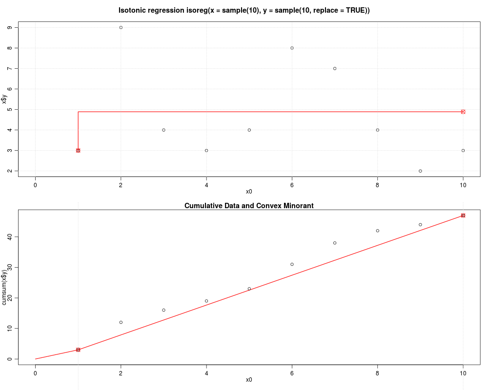
plot(ir <- isoreg(sample(10), sample(10, replace = TRUE)),
plot.type = "r")
Results
R version 3.3.1 (2016-06-21) -- "Bug in Your Hair"
Copyright (C) 2016 The R Foundation for Statistical Computing
Platform: x86_64-pc-linux-gnu (64-bit)
R is free software and comes with ABSOLUTELY NO WARRANTY.
You are welcome to redistribute it under certain conditions.
Type 'license()' or 'licence()' for distribution details.
R is a collaborative project with many contributors.
Type 'contributors()' for more information and
'citation()' on how to cite R or R packages in publications.
Type 'demo()' for some demos, 'help()' for on-line help, or
'help.start()' for an HTML browser interface to help.
Type 'q()' to quit R.
> library(stats)
> png(filename="/home/ddbj/snapshot/RGM3/R_rel/result/stats/plot.isoreg.Rd_%03d_medium.png", width=480, height=480)
> ### Name: plot.isoreg
> ### Title: Plot Method for isoreg Objects
> ### Aliases: plot.isoreg lines.isoreg
> ### Keywords: hplot print
>
> ### ** Examples
>
> require(graphics)
>
> utils::example(isoreg) # for the examples there
isoreg> require(graphics)
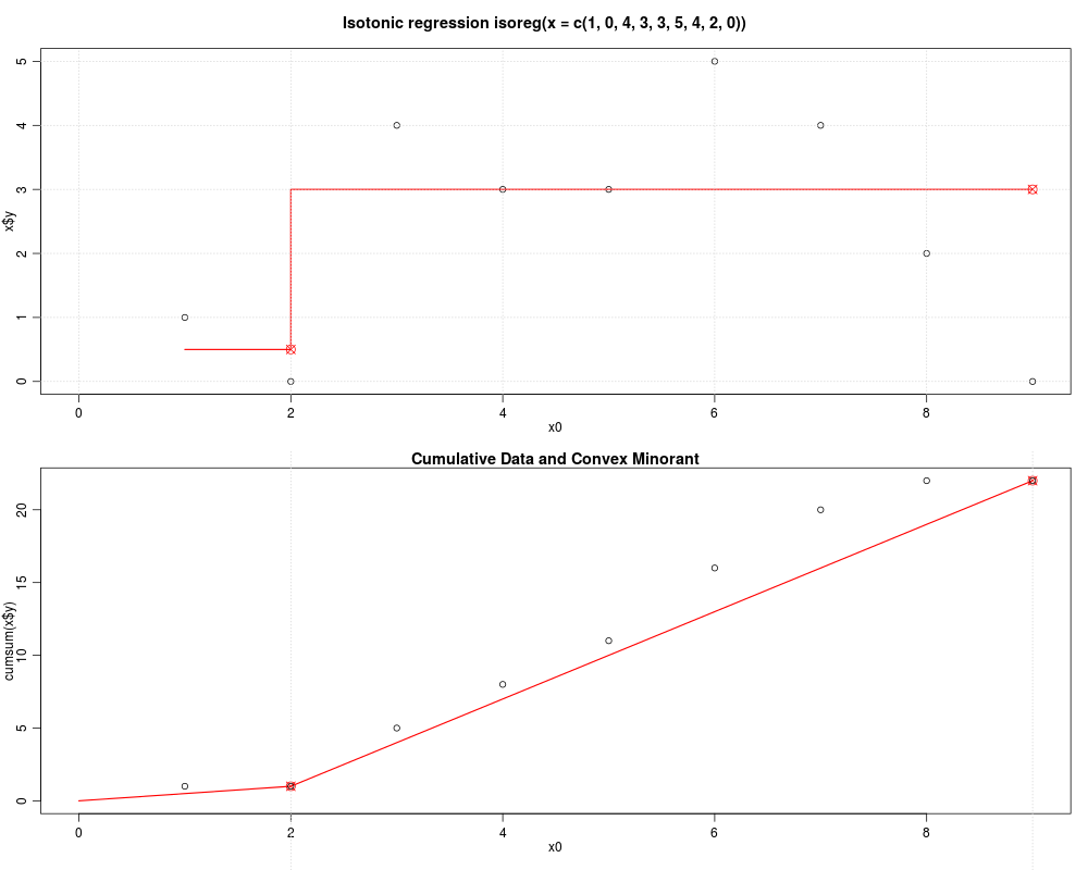
isoreg> (ir <- isoreg(c(1,0,4,3,3,5,4,2,0)))
Isotonic regression from isoreg(x = c(1, 0, 4, 3, 3, 5, 4, 2, 0)),
with 2 knots / breaks at obs.nr. 2 9 ;
initially ordered 'x'
and further components List of 4
$ x : num [1:9] 1 2 3 4 5 6 7 8 9
$ y : num [1:9] 1 0 4 3 3 5 4 2 0
$ yf: num [1:9] 0.5 0.5 3 3 3 3 3 3 3
$ yc: num [1:10] 0 1 1 5 8 11 16 20 22 22
isoreg> plot(ir, plot.type = "row")
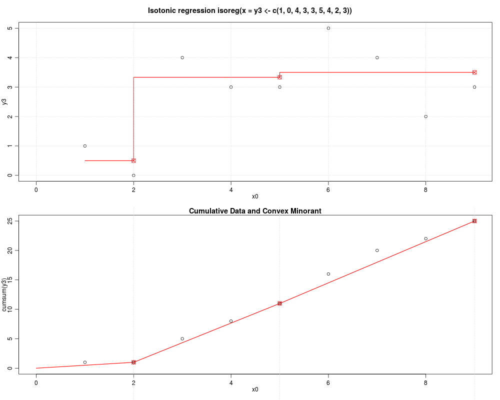
isoreg> (ir3 <- isoreg(y3 <- c(1,0,4,3,3,5,4,2, 3))) # last "3", not "0"
Isotonic regression from isoreg(x = y3 <- c(1, 0, 4, 3, 3, 5, 4, 2, 3)),
with 3 knots / breaks at obs.nr. 2 5 9 ;
initially ordered 'x'
and further components List of 4
$ x : num [1:9] 1 2 3 4 5 6 7 8 9
$ y : num [1:9] 1 0 4 3 3 5 4 2 3
$ yf: num [1:9] 0.5 0.5 3.33 3.33 3.33 ...
$ yc: num [1:10] 0 1 1 5 8 11 16 20 22 25
isoreg> (fi3 <- as.stepfun(ir3))
Step function
Call: isoreg(x = y3 <- c(1, 0, 4, 3, 3, 5, 4, 2, 3))
x[1:3] = 2, 5, 9
4 plateau levels = 0.5, 0.5, 3.3333, 3.5
isoreg> (ir4 <- isoreg(1:10, y4 <- c(5, 9, 1:2, 5:8, 3, 8)))
Isotonic regression from isoreg(x = 1:10, y = y4 <- c(5, 9, 1:2, 5:8, 3, 8)),
with 5 knots / breaks at obs.nr. 4 5 6 9 10 ;
initially ordered 'x'
and further components List of 4
$ x : num [1:10] 1 2 3 4 5 6 7 8 9 10
$ y : num [1:10] 5 9 1 2 5 6 7 8 3 8
$ yf: num [1:10] 4.25 4.25 4.25 4.25 5 6 6 6 6 8
$ yc: num [1:11] 0 5 14 15 17 22 28 35 43 46 ...
isoreg> cat(sprintf("R^2 = %.2f\n",
isoreg+ 1 - sum(residuals(ir4)^2) / ((10-1)*var(y4))))
R^2 = 0.21
isoreg> ## If you are interested in the knots alone :
isoreg> with(ir4, cbind(iKnots, yf[iKnots]))
iKnots
[1,] 4 4.25
[2,] 5 5.00
[3,] 6 6.00
[4,] 9 6.00
[5,] 10 8.00
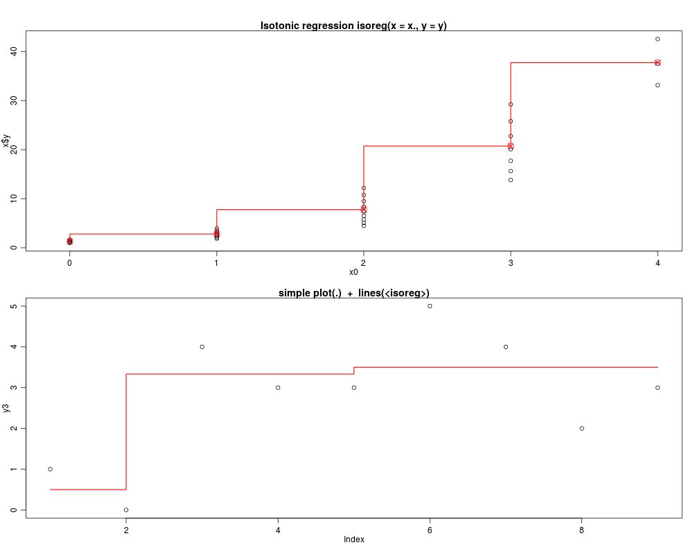
isoreg> ## Example of unordered x[] with ties:
isoreg> x <- sample((0:30)/8)
isoreg> y <- exp(x)
isoreg> x. <- round(x) # ties!
isoreg> plot(m <- isoreg(x., y))
isoreg> stopifnot(all.equal(with(m, yf[iKnots]),
isoreg+ as.vector(tapply(y, x., mean))))
>
> plot(y3, main = "simple plot(.) + lines(<isoreg>)")
> lines(ir3)
>
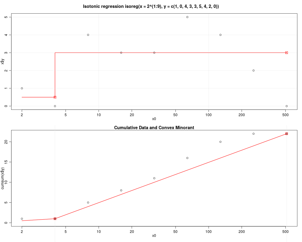
> ## 'same' plot as above, "proving" that only ranks of 'x' are important
> plot(isoreg(2^(1:9), c(1,0,4,3,3,5,4,2,0)), plot.type = "row", log = "x")
Warning messages:
1: In xy.coords(x, y, xlabel, ylabel, log) :
1 x value <= 0 omitted from logarithmic plot
2: In xy.coords(x, y, xlabel, ylabel, log) :
1 x value <= 0 omitted from logarithmic plot
>
> plot(ir3, plot.type = "row", ylab = "y3")
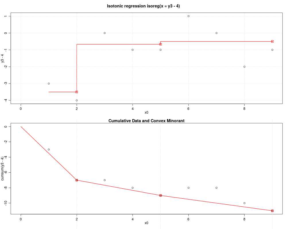
> plot(isoreg(y3 - 4), plot.t="r", ylab = "y3 - 4")
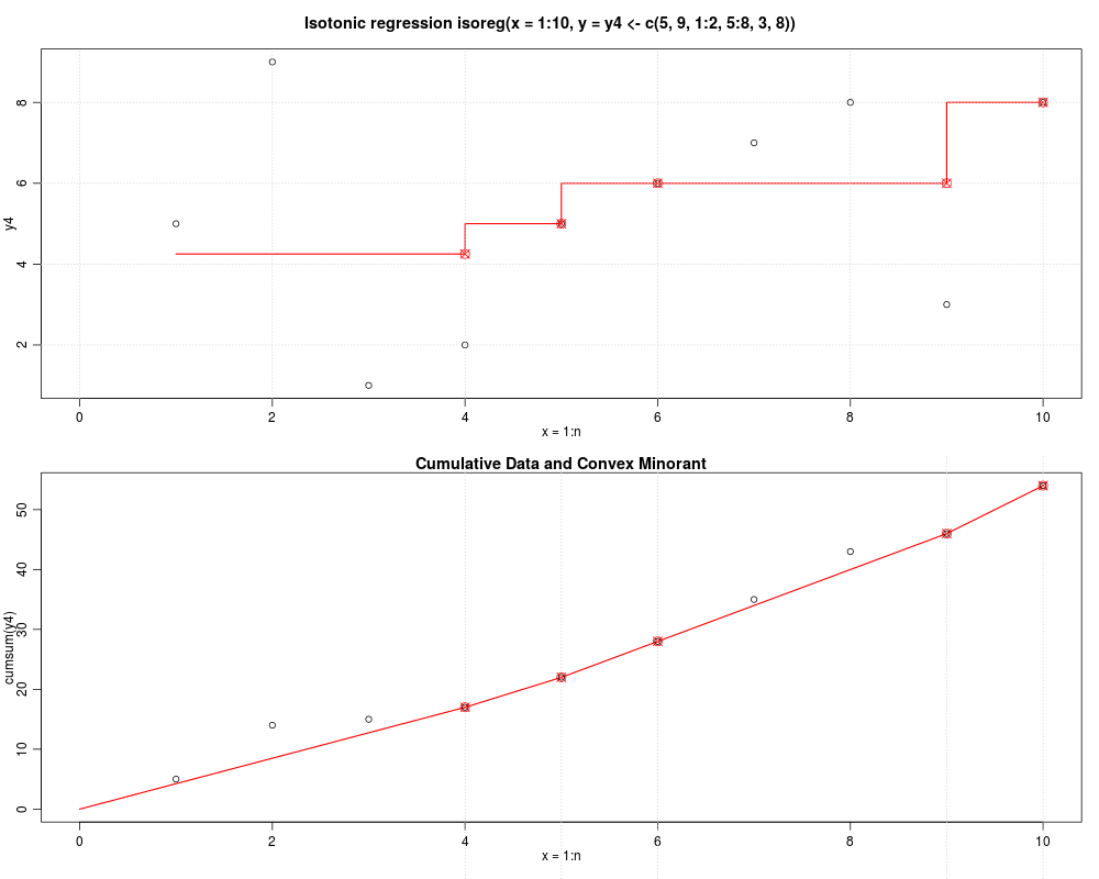
> plot(ir4, plot.type = "ro", ylab = "y4", xlab = "x = 1:n")
>
> ## experiment a bit with these (C-c C-j):
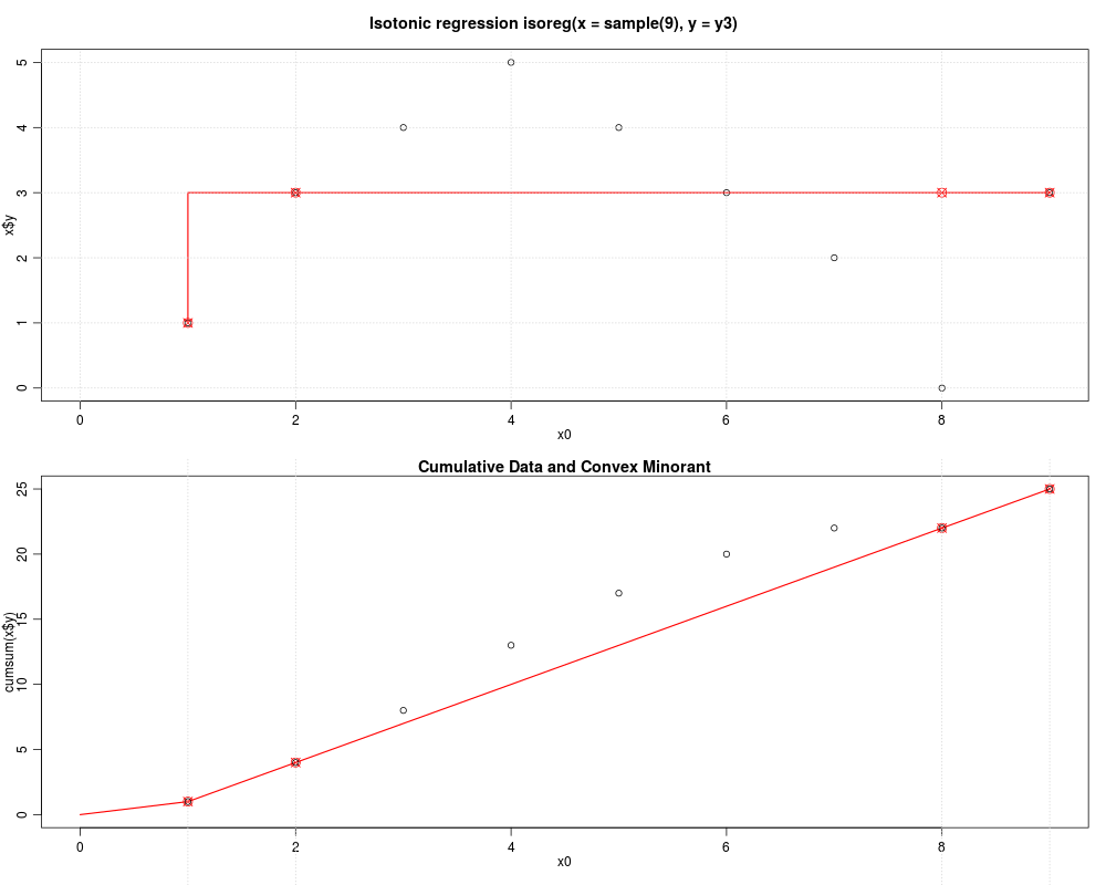
> plot(isoreg(sample(9), y3), plot.type = "row")
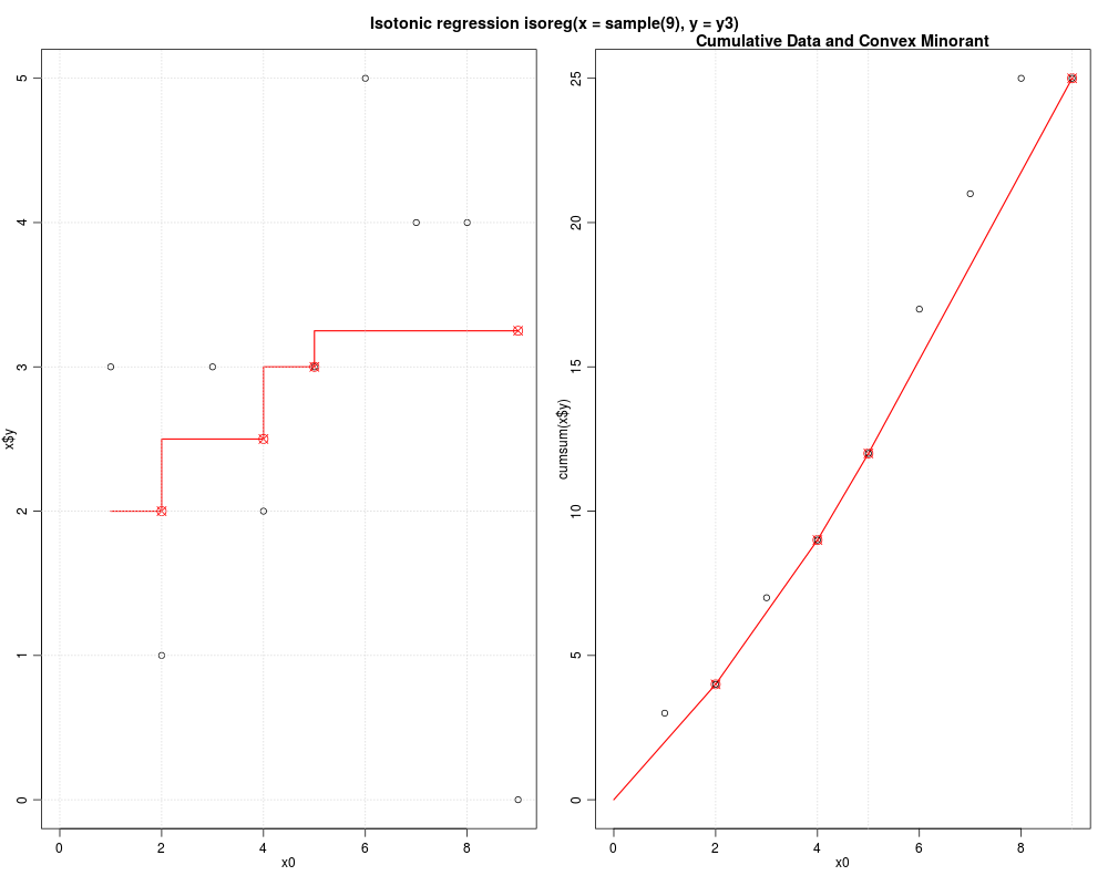
> plot(isoreg(sample(9), y3), plot.type = "col.wise")
>
> plot(ir <- isoreg(sample(10), sample(10, replace = TRUE)),
+ plot.type = "r")
>
>
>
>
>
> dev.off()
null device
1
>
 .
.