Supported by Dr. Osamu Ogasawara and  . . |
|
Last data update: 2014.03.03 |
Plot Diagnostics for an lm ObjectDescriptionSix plots (selectable by Usage
## S3 method for class 'lm'
plot(x, which = c(1:3, 5),
     caption = list("Residuals vs Fitted", "Normal Q-Q",
       "Scale-Location", "Cook's distance",
       "Residuals vs Leverage",
       expression("Cook's dist vs Leverage  " * h[ii] / (1 - h[ii]))),
     panel = if(add.smooth) panel.smooth else points,
     sub.caption = NULL, main = "",
     ask = prod(par("mfcol")) < length(which) && dev.interactive(),
     ...,
     id.n = 3, labels.id = names(residuals(x)), cex.id = 0.75,
     qqline = TRUE, cook.levels = c(0.5, 1.0),
     add.smooth = getOption("add.smooth"), label.pos = c(4,2),
     cex.caption = 1, cex.oma.main = 1.25)
Arguments
Details
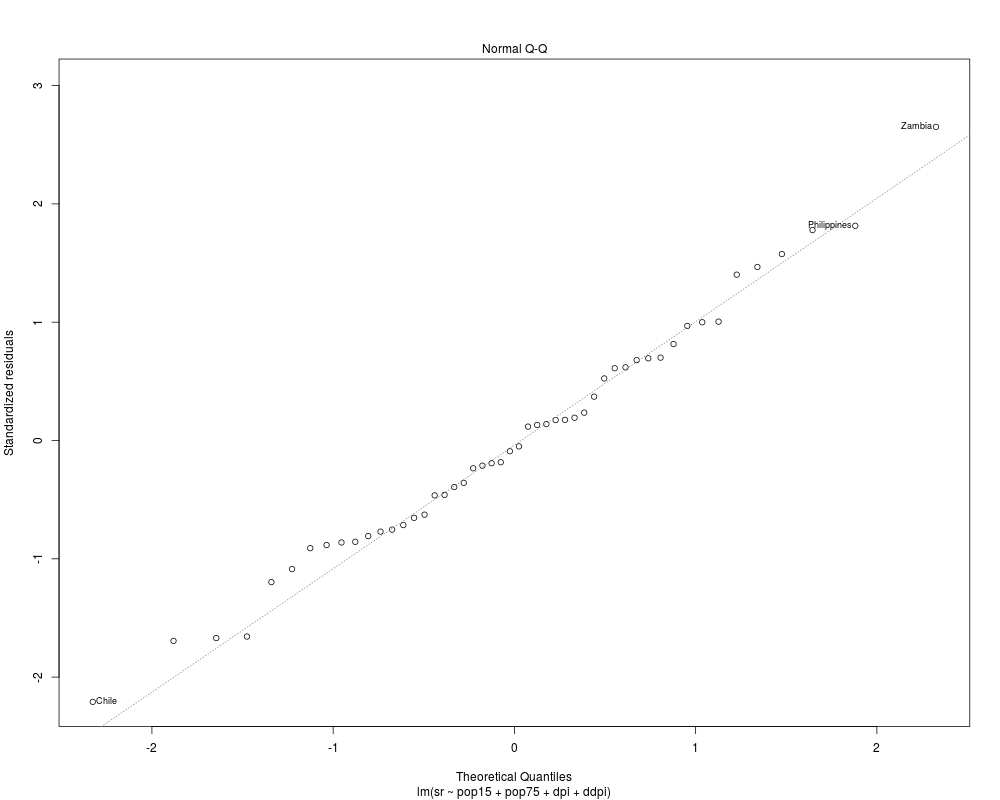
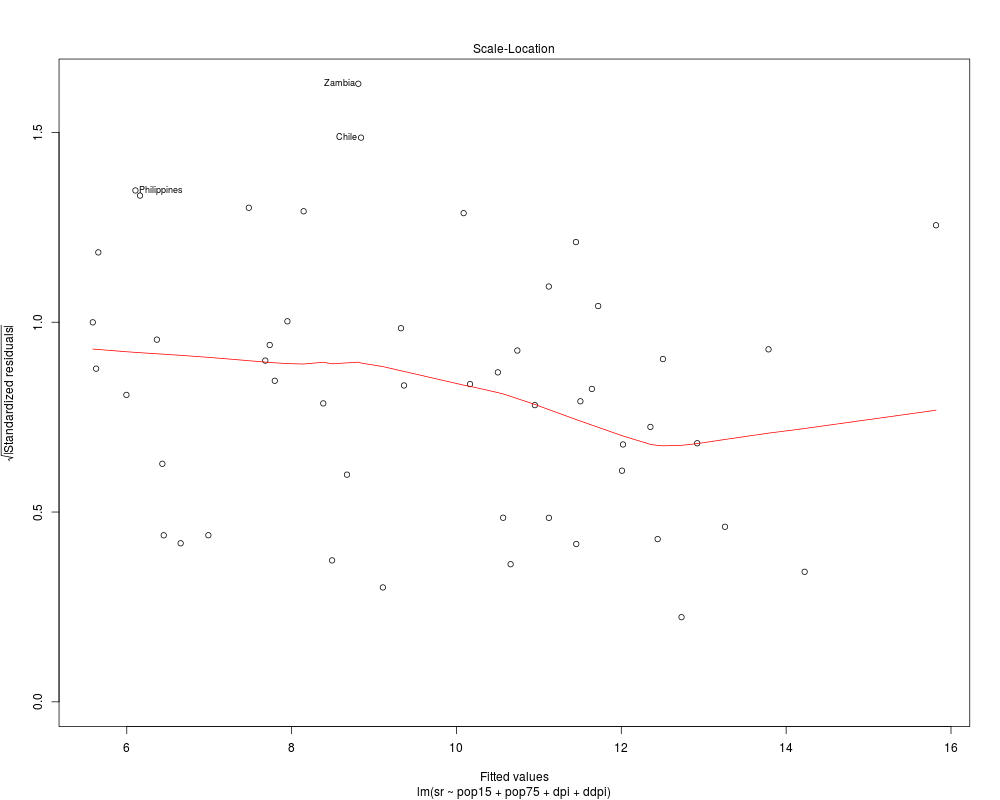
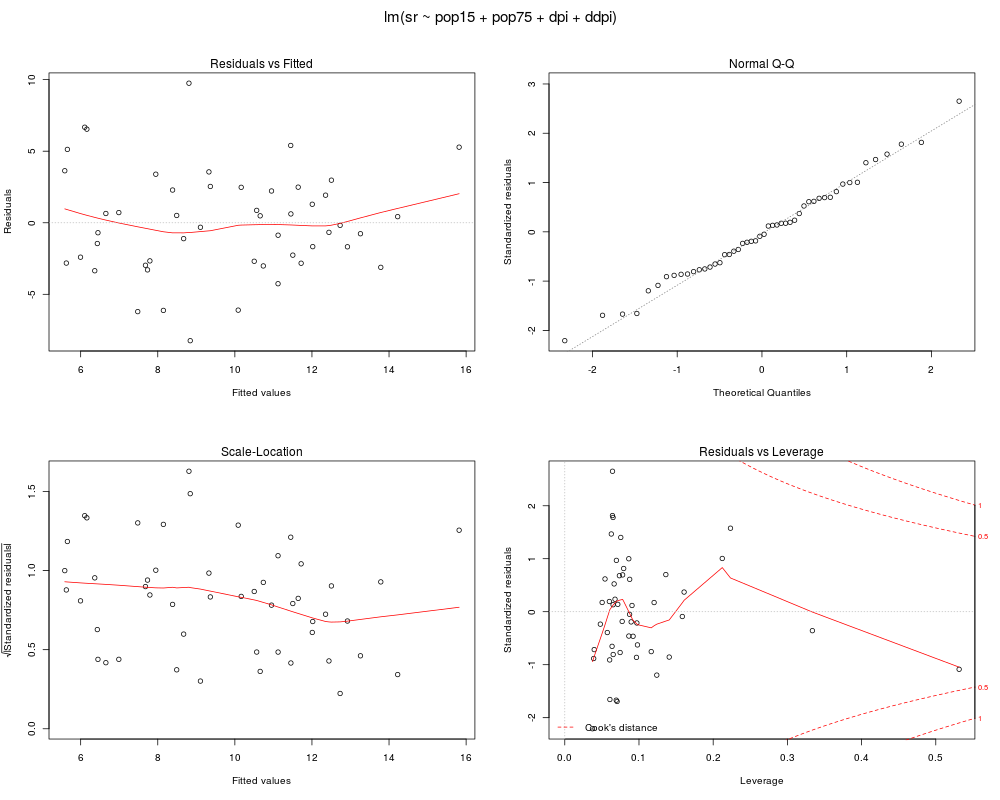
The ‘Scale-Location’ plot, also called ‘Spread-Location’ or ‘S-L’ plot, takes the square root of the absolute residuals in order to diminish skewness (sqrt(|E|)) is much less skewed than | E | for Gaussian zero-mean E). The ‘S-L’, the Q-Q, and the Residual-Leverage plot, use
standardized residuals which have identical variance (under the
hypothesis). They are given as
R[i] / (s * sqrt(1 - h.ii))
where h.ii are the diagonal entries of the hat matrix,
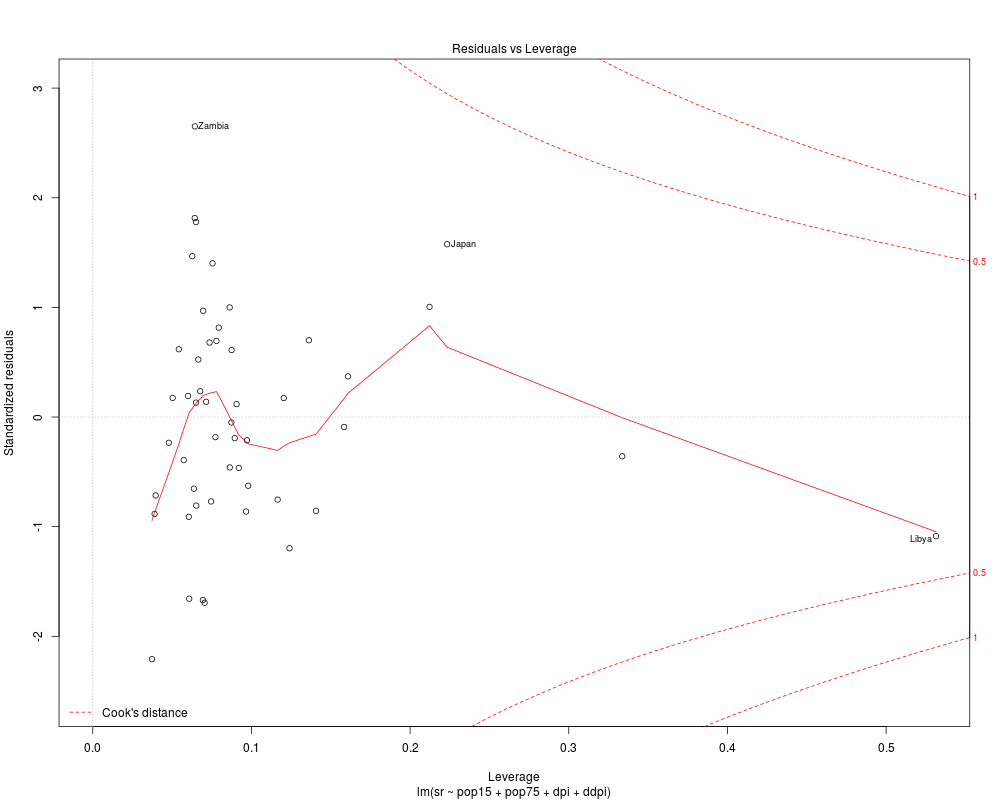
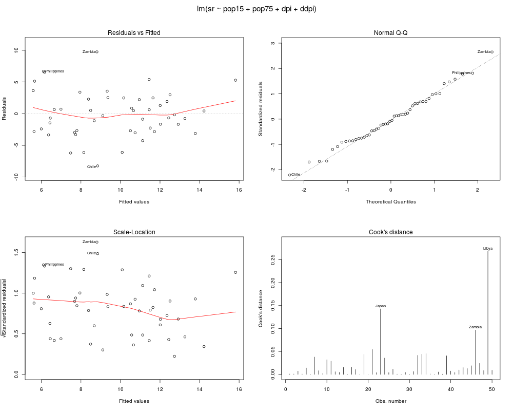
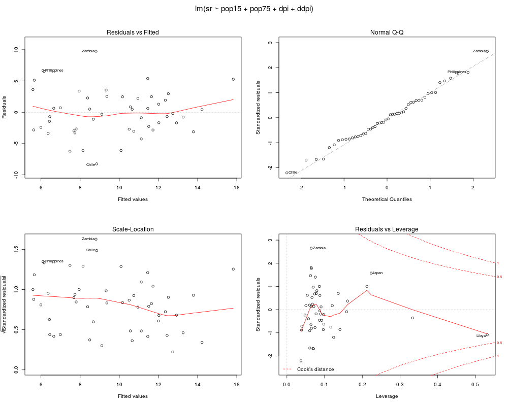
The Residual-Leverage plot shows contours of equal Cook's distance,
for values of In the Cook's distance vs leverage/(1-leverage) plot, contours of standardized residuals that are equal in magnitude are lines through the origin. The contour lines are labelled with the magnitudes. Author(s)John Maindonald and Martin Maechler. ReferencesBelsley, D. A., Kuh, E. and Welsch, R. E. (1980) Regression Diagnostics. New York: Wiley. Cook, R. D. and Weisberg, S. (1982) Residuals and Influence in Regression. London: Chapman and Hall. Firth, D. (1991) Generalized Linear Models. In Hinkley, D. V. and Reid, N. and Snell, E. J., eds: Pp. 55-82 in Statistical Theory and Modelling. In Honour of Sir David Cox, FRS. London: Chapman and Hall. Hinkley, D. V. (1975) On power transformations to symmetry. Biometrika 62, 101–111. McCullagh, P. and Nelder, J. A. (1989) Generalized Linear Models. London: Chapman and Hall. See Also
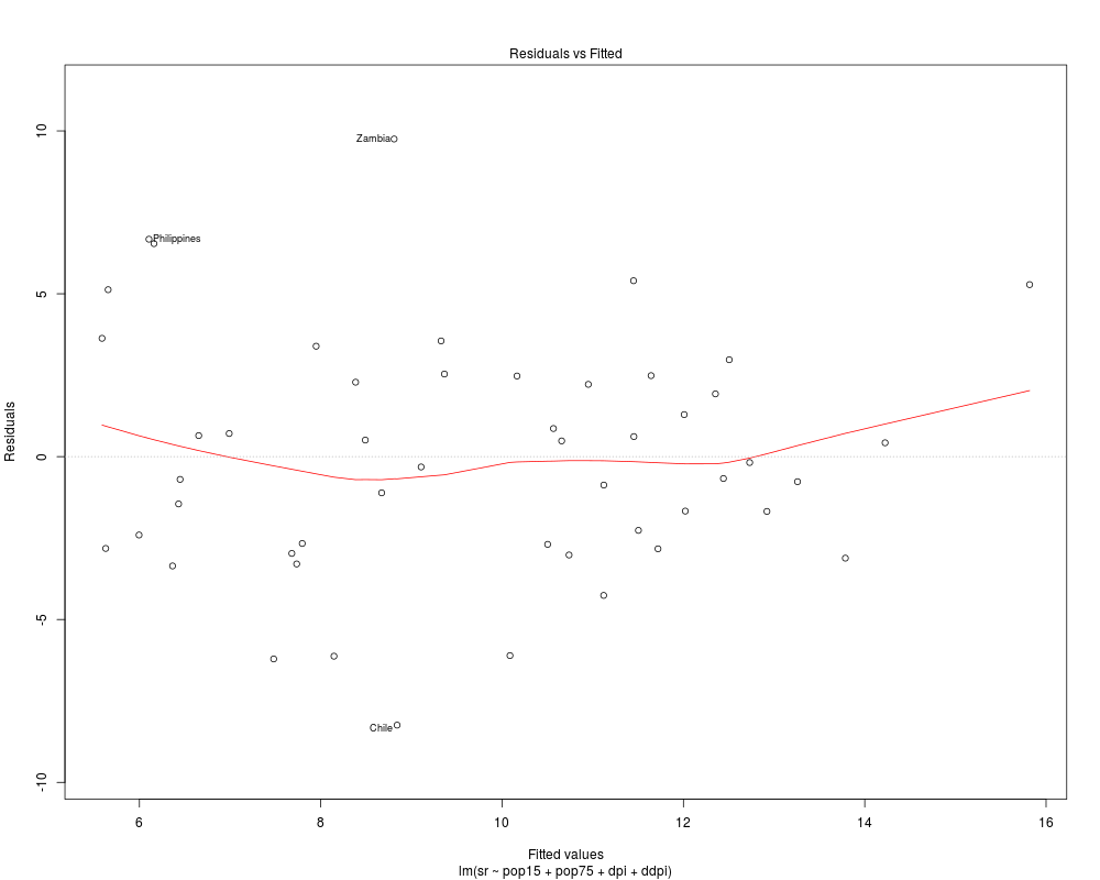
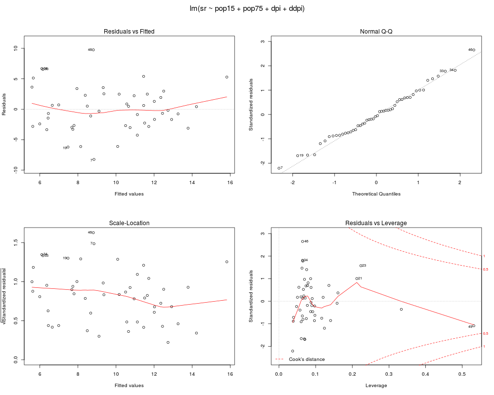
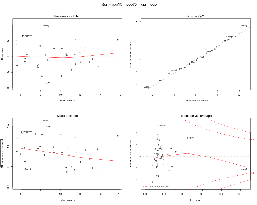
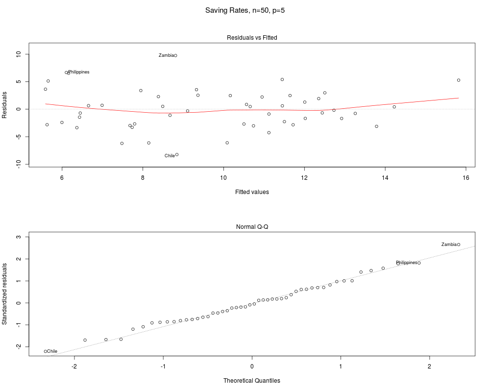
Examplesrequire(graphics) ## Analysis of the life-cycle savings data ## given in Belsley, Kuh and Welsch. lm.SR <- lm(sr ~ pop15 + pop75 + dpi + ddpi, data = LifeCycleSavings) plot(lm.SR) ## 4 plots on 1 page; ## allow room for printing model formula in outer margin: par(mfrow = c(2, 2), oma = c(0, 0, 2, 0)) plot(lm.SR) plot(lm.SR, id.n = NULL) # no id's plot(lm.SR, id.n = 5, labels.id = NULL) # 5 id numbers ## Was default in R <= 2.1.x: ## Cook's distances instead of Residual-Leverage plot plot(lm.SR, which = 1:4) ## Fit a smooth curve, where applicable: plot(lm.SR, panel = panel.smooth) ## Gives a smoother curve plot(lm.SR, panel = function(x, y) panel.smooth(x, y, span = 1)) par(mfrow = c(2,1)) # same oma as above plot(lm.SR, which = 1:2, sub.caption = "Saving Rates, n=50, p=5") Results
R version 3.3.1 (2016-06-21) -- "Bug in Your Hair"
Copyright (C) 2016 The R Foundation for Statistical Computing
Platform: x86_64-pc-linux-gnu (64-bit)
R is free software and comes with ABSOLUTELY NO WARRANTY.
You are welcome to redistribute it under certain conditions.
Type 'license()' or 'licence()' for distribution details.
R is a collaborative project with many contributors.
Type 'contributors()' for more information and
'citation()' on how to cite R or R packages in publications.
Type 'demo()' for some demos, 'help()' for on-line help, or
'help.start()' for an HTML browser interface to help.
Type 'q()' to quit R.
> library(stats)
> png(filename="/home/ddbj/snapshot/RGM3/R_rel/result/stats/plot.lm.Rd_%03d_medium.png", width=480, height=480)
> ### Name: plot.lm
> ### Title: Plot Diagnostics for an lm Object
> ### Aliases: plot.lm
> ### Keywords: hplot regression
>
> ### ** Examples
>
> require(graphics)
>
> ## Analysis of the life-cycle savings data
> ## given in Belsley, Kuh and Welsch.
> lm.SR <- lm(sr ~ pop15 + pop75 + dpi + ddpi, data = LifeCycleSavings)
> plot(lm.SR)
>
> ## 4 plots on 1 page;
> ## allow room for printing model formula in outer margin:
> par(mfrow = c(2, 2), oma = c(0, 0, 2, 0))
> plot(lm.SR)
> plot(lm.SR, id.n = NULL) # no id's
> plot(lm.SR, id.n = 5, labels.id = NULL) # 5 id numbers
>
> ## Was default in R <= 2.1.x:
> ## Cook's distances instead of Residual-Leverage plot
> plot(lm.SR, which = 1:4)
>
> ## Fit a smooth curve, where applicable:
> plot(lm.SR, panel = panel.smooth)
> ## Gives a smoother curve
> plot(lm.SR, panel = function(x, y) panel.smooth(x, y, span = 1))
>
> par(mfrow = c(2,1)) # same oma as above
> plot(lm.SR, which = 1:2, sub.caption = "Saving Rates, n=50, p=5")
>
> ## Don't show:
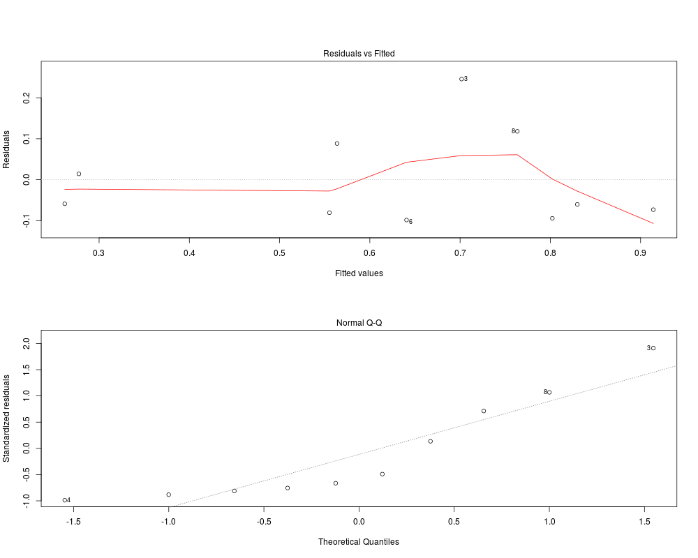
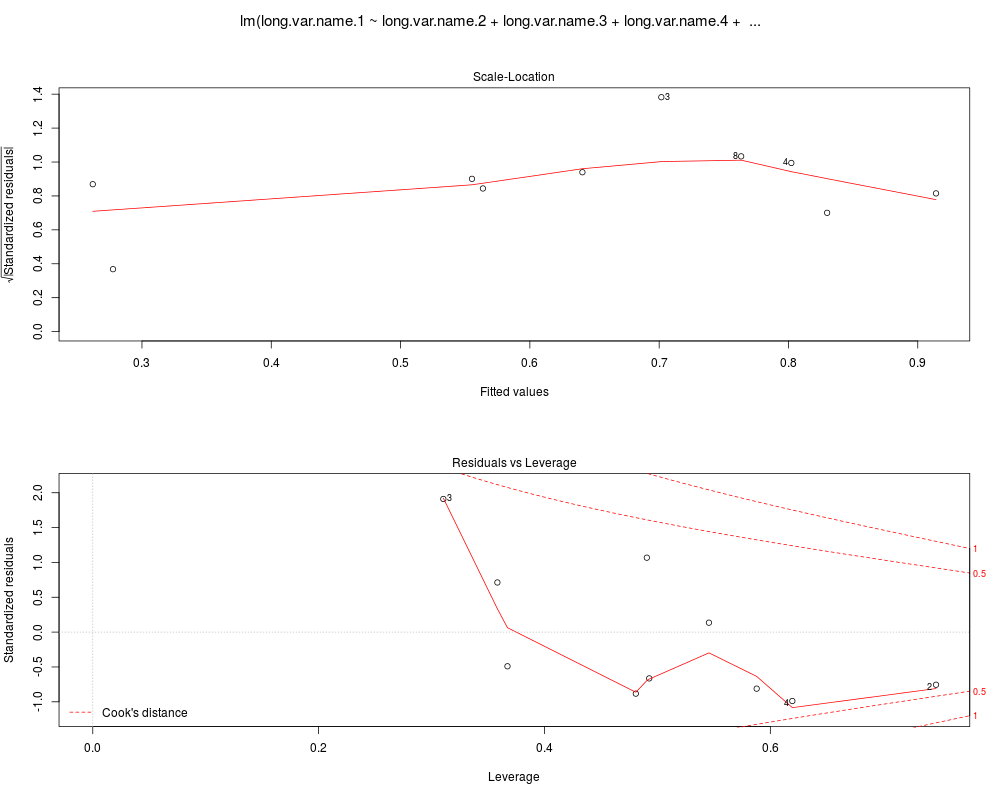
> ## An example with *long* formula that needs abbreviation:
> for(i in 1:5) assign(paste("long.var.name", i, sep = "."), runif(10))
> plot(lm(long.var.name.1 ~
+ long.var.name.2 + long.var.name.3 + long.var.name.4 + long.var.name.5))
> ## End(Don't show)
>
>
>
>
>
> dev.off()
null device
1
>
|