Supported by Dr. Osamu Ogasawara and  . . |
|
Last data update: 2014.03.03 |
Plotting Time-Series ObjectsDescriptionPlotting method for objects inheriting from class Usage
## S3 method for class 'ts'
plot(x, y = NULL, plot.type = c("multiple", "single"),
        xy.labels, xy.lines, panel = lines, nc, yax.flip = FALSE,
        mar.multi = c(0, 5.1, 0, if(yax.flip) 5.1 else 2.1),
        oma.multi = c(6, 0, 5, 0), axes = TRUE, ...)

## S3 method for class 'ts'
lines(x, ...)
Arguments
DetailsIf If See Also
Examples
require(graphics)
## Multivariate
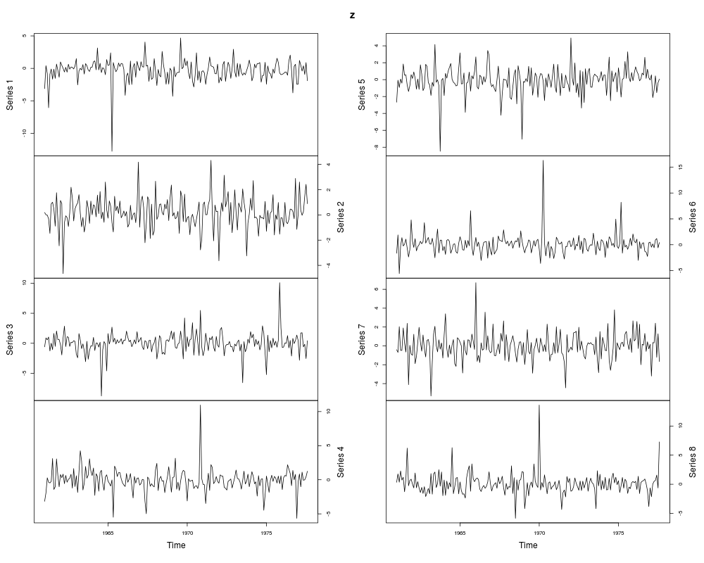
z <- ts(matrix(rt(200 * 8, df = 3), 200, 8),
start = c(1961, 1), frequency = 12)
plot(z, yax.flip = TRUE)
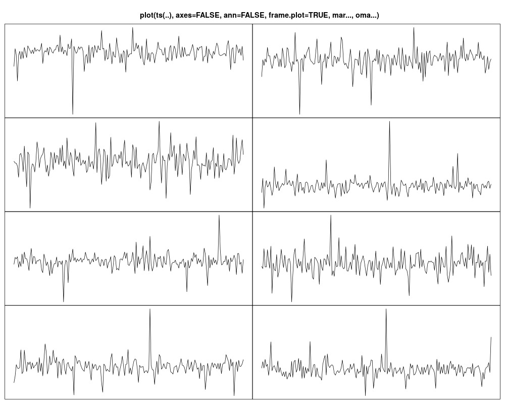
plot(z, axes = FALSE, ann = FALSE, frame.plot = TRUE,
mar.multi = c(0,0,0,0), oma.multi = c(1,1,5,1))
title("plot(ts(..), axes=FALSE, ann=FALSE, frame.plot=TRUE, mar..., oma...)")
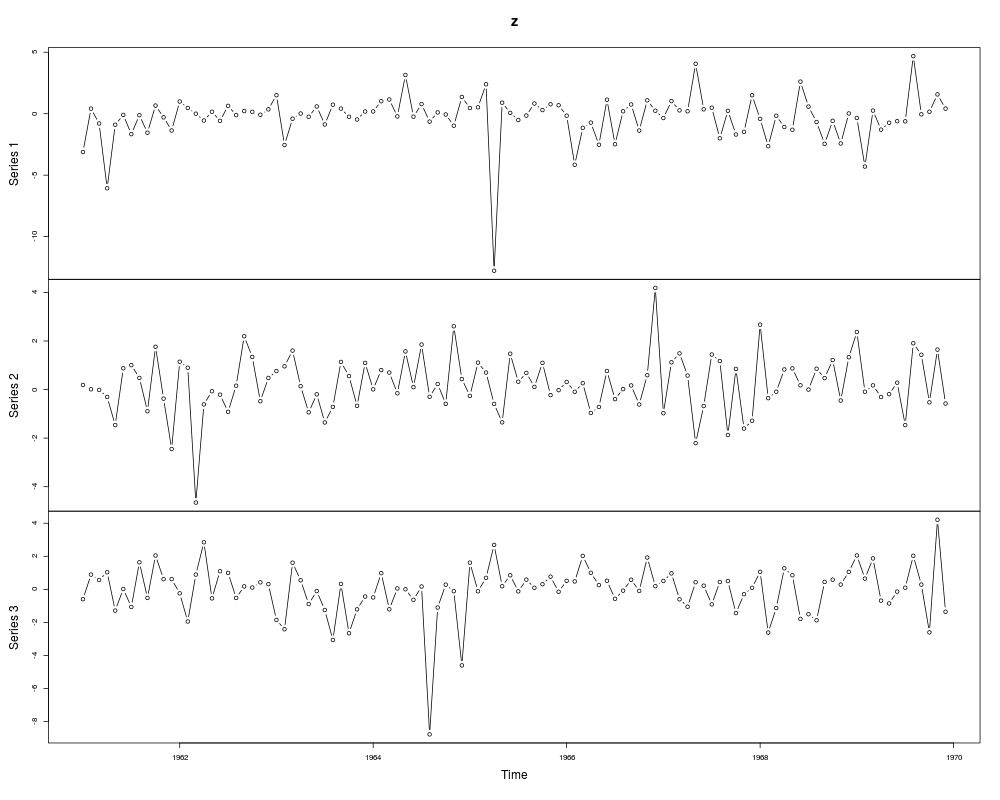
z <- window(z[,1:3], end = c(1969,12))
plot(z, type = "b") # multiple
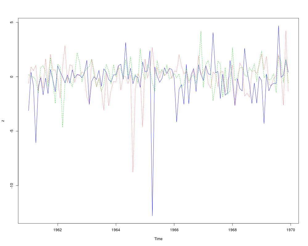
plot(z, plot.type = "single", lty = 1:3, col = 4:2)
## A phase plot:
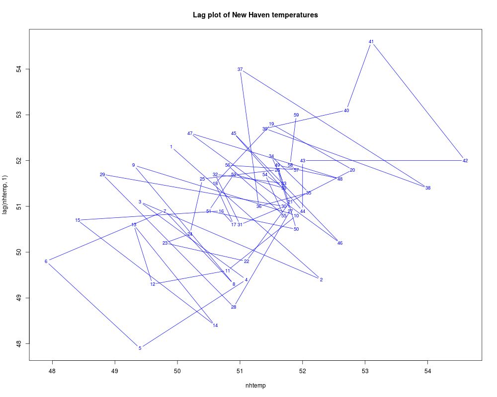
plot(nhtemp, lag(nhtemp, 1), cex = .8, col = "blue",
main = "Lag plot of New Haven temperatures")
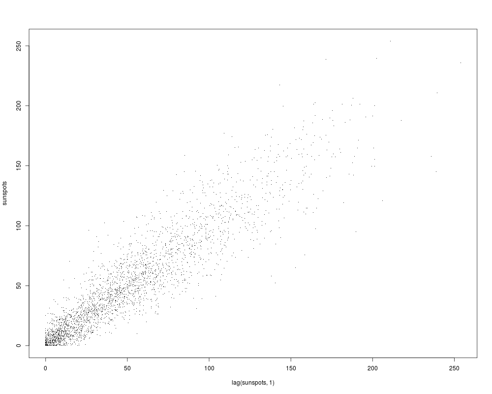
## xy.lines and xy.labels are FALSE for large series:
plot(lag(sunspots, 1), sunspots, pch = ".")
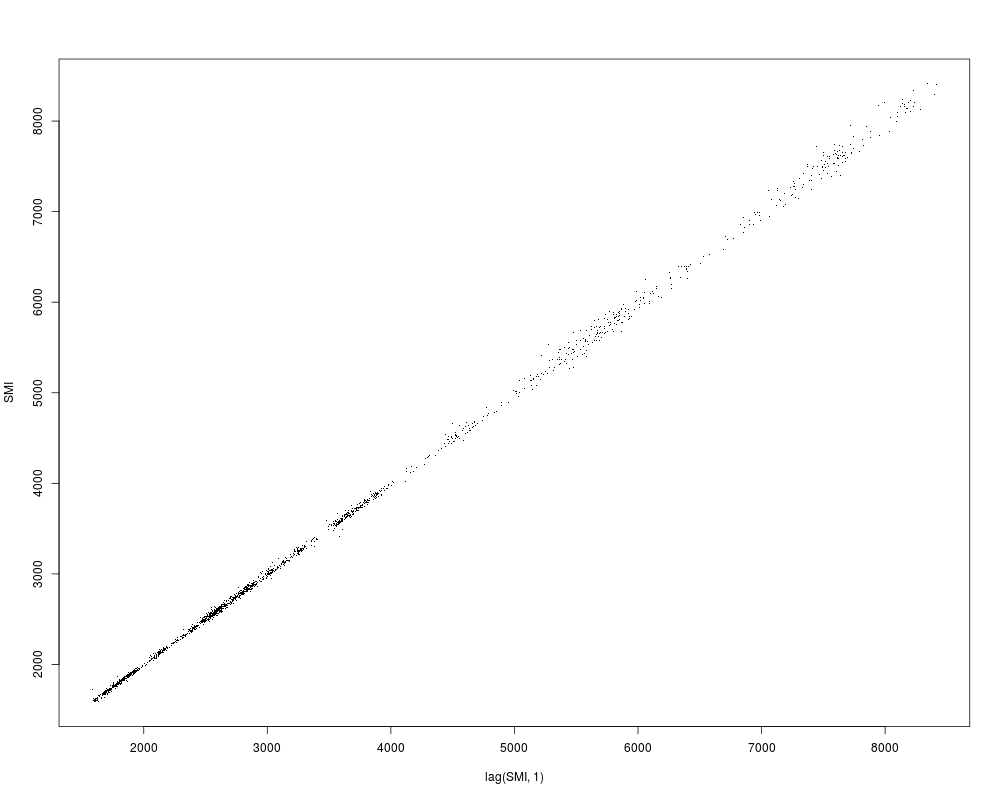
SMI <- EuStockMarkets[, "SMI"]
plot(lag(SMI, 1), SMI, pch = ".")
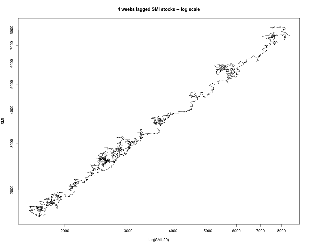
plot(lag(SMI, 20), SMI, pch = ".", log = "xy",
main = "4 weeks lagged SMI stocks -- log scale", xy.lines = TRUE)
Results
R version 3.3.1 (2016-06-21) -- "Bug in Your Hair"
Copyright (C) 2016 The R Foundation for Statistical Computing
Platform: x86_64-pc-linux-gnu (64-bit)

R is free software and comes with ABSOLUTELY NO WARRANTY.
You are welcome to redistribute it under certain conditions.
Type 'license()' or 'licence()' for distribution details.

R is a collaborative project with many contributors.
Type 'contributors()' for more information and
'citation()' on how to cite R or R packages in publications.

Type 'demo()' for some demos, 'help()' for on-line help, or
'help.start()' for an HTML browser interface to help.
Type 'q()' to quit R.

> library(stats)
> png(filename="/home/ddbj/snapshot/RGM3/R_rel/result/stats/plot.ts.Rd_%03d_medium.png", width=480, height=480)
> ### Name: plot.ts
> ### Title: Plotting Time-Series Objects
> ### Aliases: plot.ts lines.ts
> ### Keywords: hplot ts
>
> ### ** Examples
>
> require(graphics)
>
> ## Multivariate
> z <- ts(matrix(rt(200 * 8, df = 3), 200, 8),
+         start = c(1961, 1), frequency = 12)
> plot(z, yax.flip = TRUE)
> plot(z, axes = FALSE, ann = FALSE, frame.plot = TRUE,
+      mar.multi = c(0,0,0,0), oma.multi = c(1,1,5,1))
> title("plot(ts(..), axes=FALSE, ann=FALSE, frame.plot=TRUE, mar..., oma...)")
>
> z <- window(z[,1:3], end = c(1969,12))
> plot(z, type = "b")    # multiple
> plot(z, plot.type = "single", lty = 1:3, col = 4:2)
>
> ## A phase plot:
> plot(nhtemp, lag(nhtemp, 1), cex = .8, col = "blue",
+      main = "Lag plot of New Haven temperatures")
>
> ## xy.lines and xy.labels are FALSE for large series:
> plot(lag(sunspots, 1), sunspots, pch = ".")
>
> SMI <- EuStockMarkets[, "SMI"]
> plot(lag(SMI,  1), SMI, pch = ".")
> plot(lag(SMI, 20), SMI, pch = ".", log = "xy",
+      main = "4 weeks lagged SMI stocks -- log scale", xy.lines =  TRUE)
>
>
>
>
>
> dev.off()
null device
          1
>
|