Supported by Dr. Osamu Ogasawara and  . . |
|
Last data update: 2014.03.03 |
Running Medians – Robust Scatter Plot SmoothingDescriptionCompute running medians of odd span. This is the ‘most robust’ scatter plot smoothing possible. For efficiency (and historical reason), you can use one of two different algorithms giving identical results. Usage
runmed(x, k, endrule = c("median", "keep", "constant"),
       algorithm = NULL, print.level = 0)
Arguments
DetailsApart from the end values, the result The two algorithms are internally entirely different:
Currently long vectors are only supported for Valuevector of smoothed values of the same length as Author(s)Martin Maechler maechler@stat.math.ethz.ch, based on Fortran code from Werner Stuetzle and S-PLUS and C code from Berwin Turlach. ReferencesHärdle, W. and Steiger, W. (1995) [Algorithm AS 296] Optimal median smoothing, Applied Statistics 44, 258–264. Jerome H. Friedman and Werner Stuetzle (1982) Smoothing of Scatterplots; Report, Dep. Statistics, Stanford U., Project Orion 003. Martin Maechler (2003) Fast Running Medians: Finite Sample and Asymptotic Optimality; working paper available from the author. See Also
Examples
require(graphics)
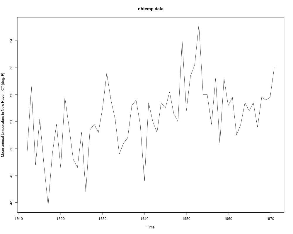
utils::example(nhtemp)
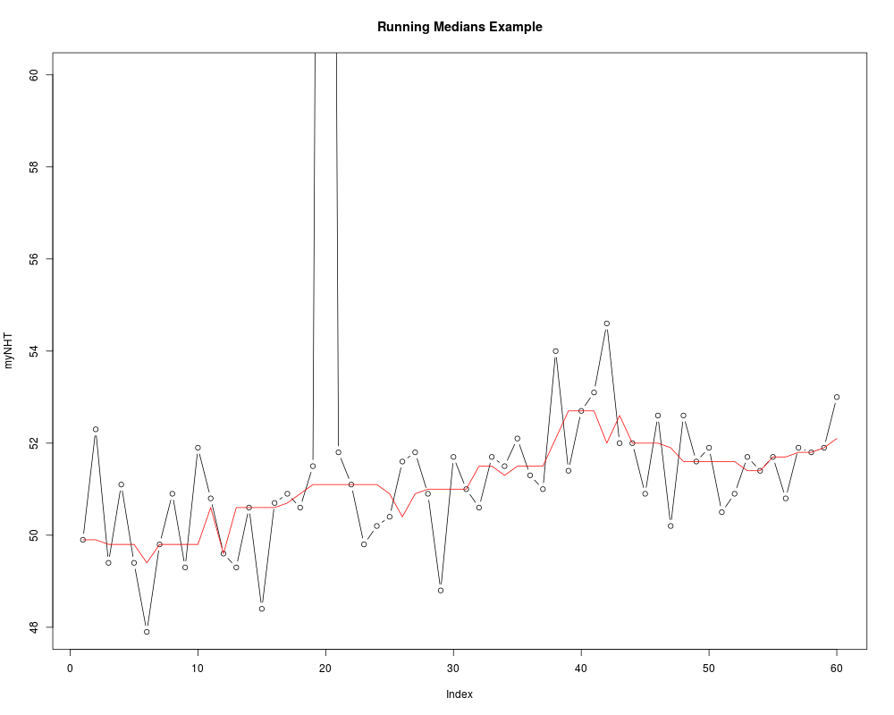
myNHT <- as.vector(nhtemp)
myNHT[20] <- 2 * nhtemp[20]
plot(myNHT, type = "b", ylim = c(48, 60), main = "Running Medians Example")
lines(runmed(myNHT, 7), col = "red")
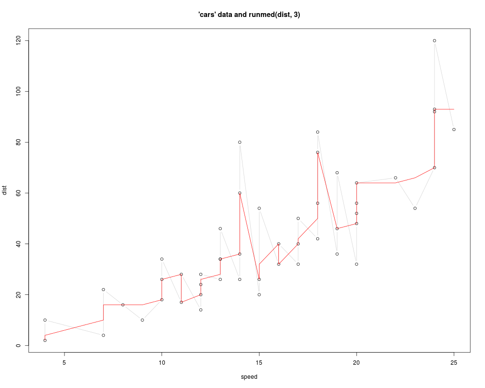
## special: multiple y values for one x
plot(cars, main = "'cars' data and runmed(dist, 3)")
lines(cars, col = "light gray", type = "c")
with(cars, lines(speed, runmed(dist, k = 3), col = 2))
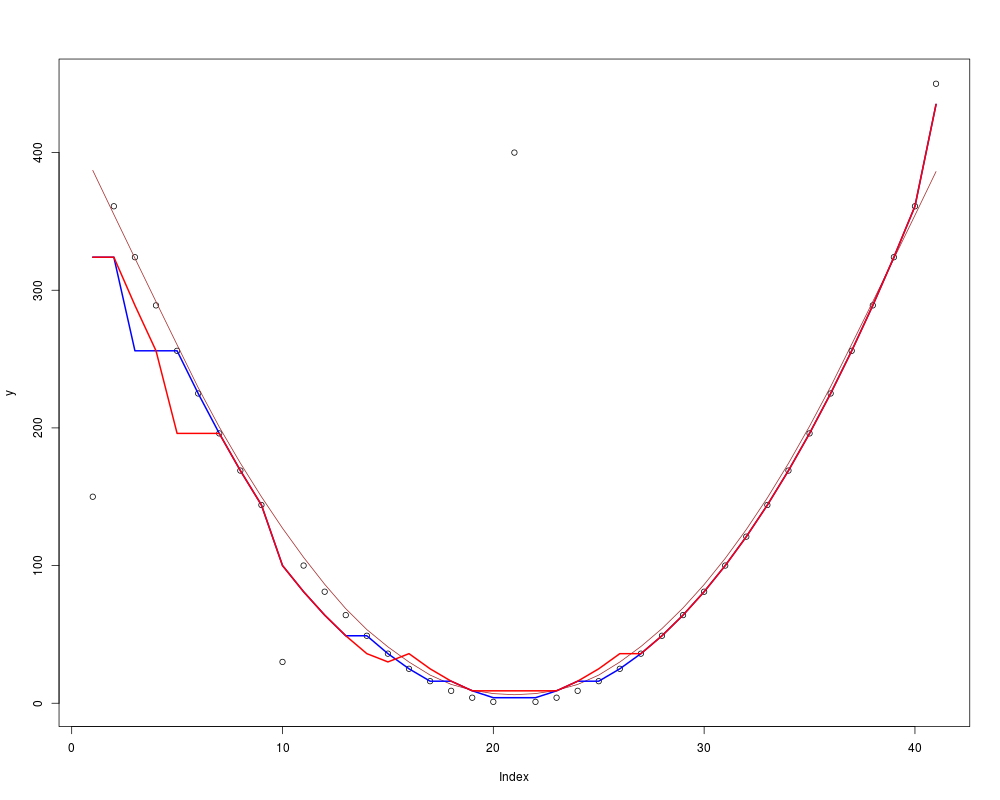
## nice quadratic with a few outliers
y <- ys <- (-20:20)^2
y [c(1,10,21,41)] <- c(150, 30, 400, 450)
all(y == runmed(y, 1)) # 1-neighbourhood <==> interpolation
plot(y) ## lines(y, lwd = .1, col = "light gray")
lines(lowess(seq(y), y, f = 0.3), col = "brown")
lines(runmed(y, 7), lwd = 2, col = "blue")
lines(runmed(y, 11), lwd = 2, col = "red")
## Lowess is not robust
y <- ys ; y[21] <- 6666 ; x <- seq(y)
col <- c("black", "brown","blue")
plot(y, col = col[1])
lines(lowess(x, y, f = 0.3), col = col[2])
lines(runmed(y, 7), lwd = 2, col = col[3])
legend(length(y),max(y), c("data", "lowess(y, f = 0.3)", "runmed(y, 7)"),
xjust = 1, col = col, lty = c(0, 1, 1), pch = c(1,NA,NA))
Results
R version 3.3.1 (2016-06-21) -- "Bug in Your Hair"
Copyright (C) 2016 The R Foundation for Statistical Computing
Platform: x86_64-pc-linux-gnu (64-bit)

R is free software and comes with ABSOLUTELY NO WARRANTY.
You are welcome to redistribute it under certain conditions.
Type 'license()' or 'licence()' for distribution details.

R is a collaborative project with many contributors.
Type 'contributors()' for more information and
'citation()' on how to cite R or R packages in publications.

Type 'demo()' for some demos, 'help()' for on-line help, or
'help.start()' for an HTML browser interface to help.
Type 'q()' to quit R.

> library(stats)
> png(filename="/home/ddbj/snapshot/RGM3/R_rel/result/stats/runmed.Rd_%03d_medium.png", width=480, height=480)
> ### Name: runmed
> ### Title: Running Medians - Robust Scatter Plot Smoothing
> ### Aliases: runmed
> ### Keywords: smooth robust
>
> ### ** Examples
>
> require(graphics)
>
> utils::example(nhtemp)

nhtemp> require(stats); require(graphics)

nhtemp> plot(nhtemp, main = "nhtemp data",
nhtemp+   ylab = "Mean annual temperature in New Haven, CT (deg. F)")
> myNHT <- as.vector(nhtemp)
> myNHT[20] <- 2 * nhtemp[20]
> plot(myNHT, type = "b", ylim = c(48, 60), main = "Running Medians Example")
> lines(runmed(myNHT, 7), col = "red")
>
> ## special: multiple y values for one x
> plot(cars, main = "'cars' data and runmed(dist, 3)")
> lines(cars, col = "light gray", type = "c")
> with(cars, lines(speed, runmed(dist, k = 3), col = 2))
>
> ## nice quadratic with a few outliers
> y <- ys <- (-20:20)^2
> y [c(1,10,21,41)] <- c(150, 30, 400, 450)
> all(y == runmed(y, 1)) # 1-neighbourhood <==> interpolation
[1] TRUE
> plot(y) ## lines(y, lwd = .1, col = "light gray")
> lines(lowess(seq(y), y, f = 0.3), col = "brown")
> lines(runmed(y, 7), lwd = 2, col = "blue")
> lines(runmed(y, 11), lwd = 2, col = "red")
>
> ## Lowess is not robust
> y <- ys ; y[21] <- 6666 ; x <- seq(y)
> col <- c("black", "brown","blue")
> plot(y, col = col[1])
> lines(lowess(x, y, f = 0.3), col = col[2])
> lines(runmed(y, 7),      lwd = 2, col = col[3])
> legend(length(y),max(y), c("data", "lowess(y, f = 0.3)", "runmed(y, 7)"),
+        xjust = 1, col = col, lty = c(0, 1, 1), pch = c(1,NA,NA))
>
>
>
>
>
> dev.off()
null device
          1
>
|