Supported by Dr. Osamu Ogasawara and  . . |
|
Last data update: 2014.03.03 |
Estimate Spectral Density of a Time Series by a Smoothed PeriodogramDescription
Usage
spec.pgram(x, spans = NULL, kernel, taper = 0.1,
           pad = 0, fast = TRUE, demean = FALSE, detrend = TRUE,
           plot = TRUE, na.action = na.fail, ...)
Arguments
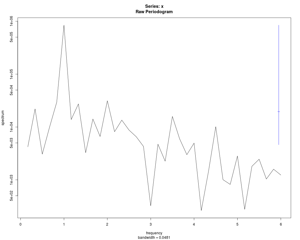
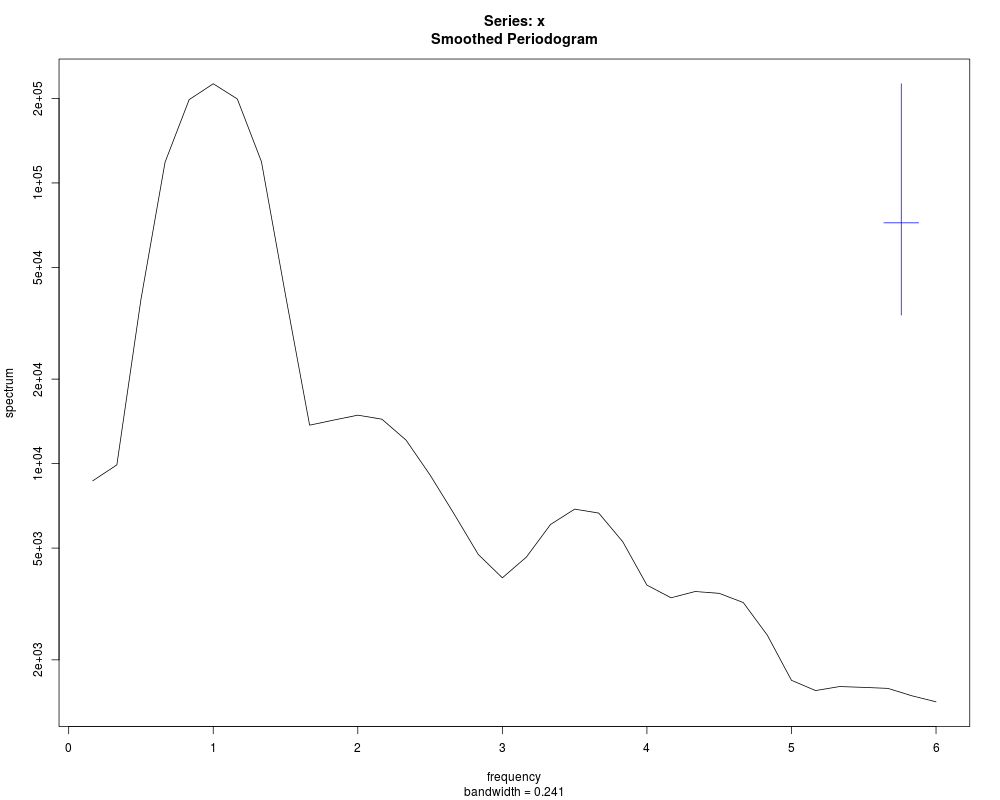
DetailsThe raw periodogram is not a consistent estimator of the spectral density, but adjacent values are asymptotically independent. Hence a consistent estimator can be derived by smoothing the raw periodogram, assuming that the spectral density is smooth. The series will be automatically padded with zeros until the series
length is a highly composite number in order to help the Fast Fourier
Transform. This is controlled by the The periodogram at zero is in theory zero as the mean of the series is removed (but this may be affected by tapering): it is replaced by an interpolation of adjacent values during smoothing, and no value is returned for that frequency. ValueA list object of class
The result is returned invisibly if Author(s)Originally Martyn Plummer; kernel smoothing by Adrian Trapletti, synthesis by B.D. Ripley ReferencesBloomfield, P. (1976) Fourier Analysis of Time Series: An Introduction. Wiley. Brockwell, P.J. and Davis, R.A. (1991) Time Series: Theory and Methods. Second edition. Springer. Venables, W.N. and Ripley, B.D. (2002) Modern Applied Statistics with S. Fourth edition. Springer. (Especially pp. 392–7.) See Also
Examples
require(graphics)
## Examples from Venables & Ripley
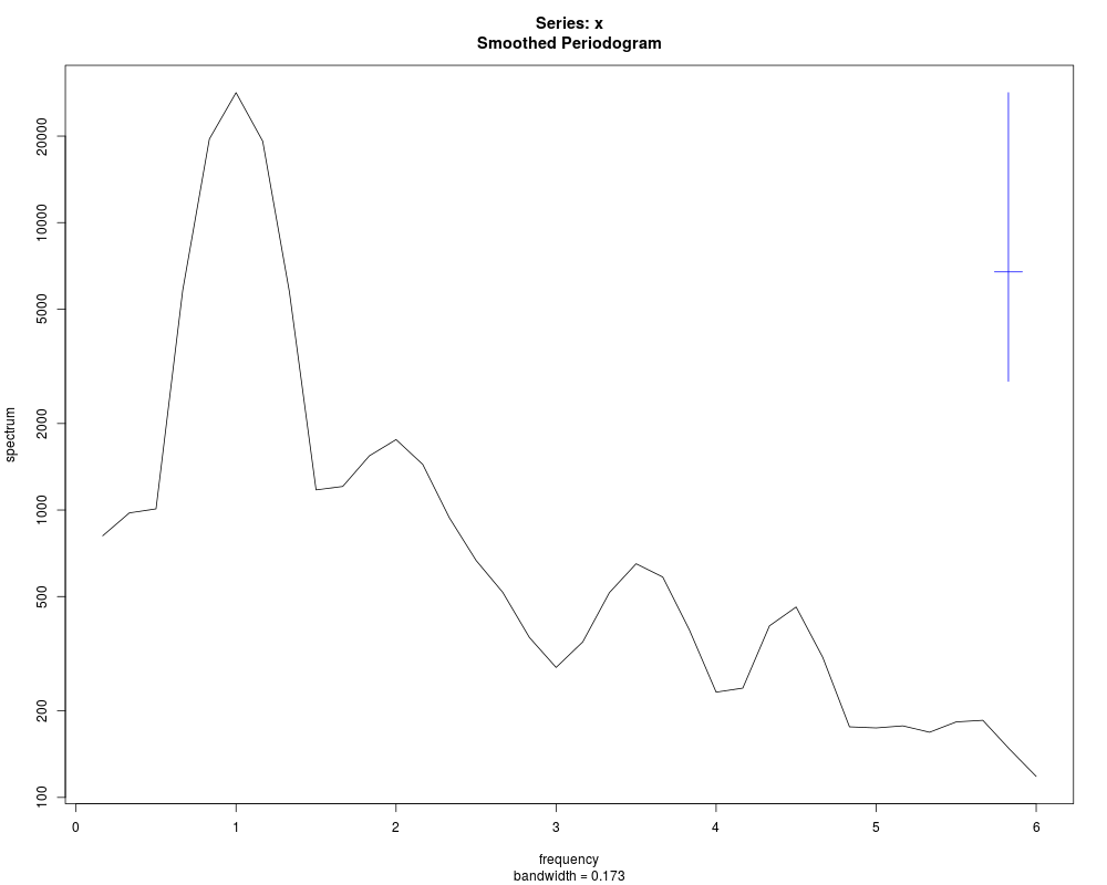
spectrum(ldeaths)
spectrum(ldeaths, spans = c(3,5))
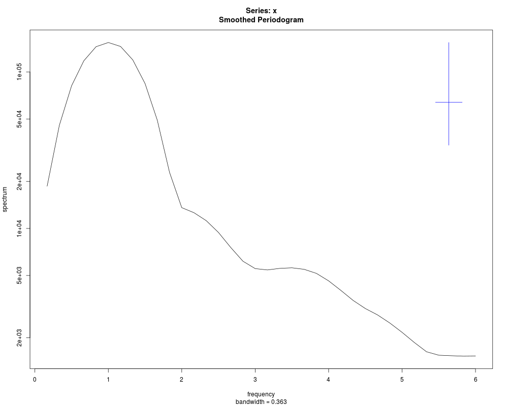
spectrum(ldeaths, spans = c(5,7))
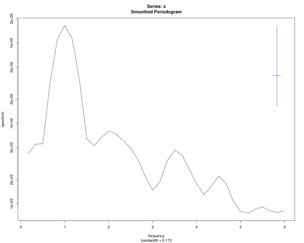
spectrum(mdeaths, spans = c(3,3))
spectrum(fdeaths, spans = c(3,3))
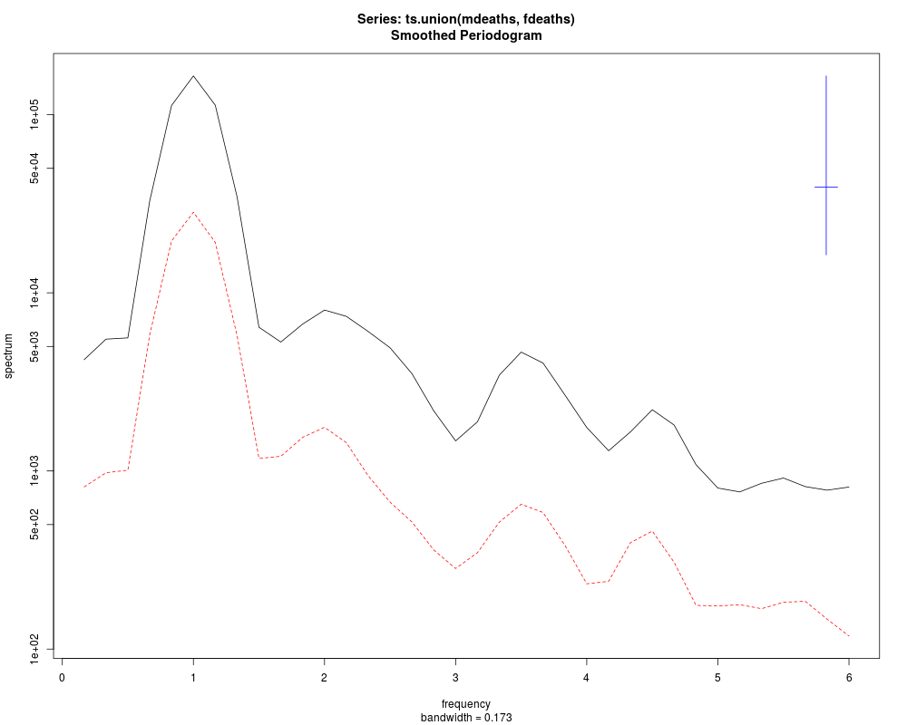
## bivariate example
mfdeaths.spc <- spec.pgram(ts.union(mdeaths, fdeaths), spans = c(3,3))
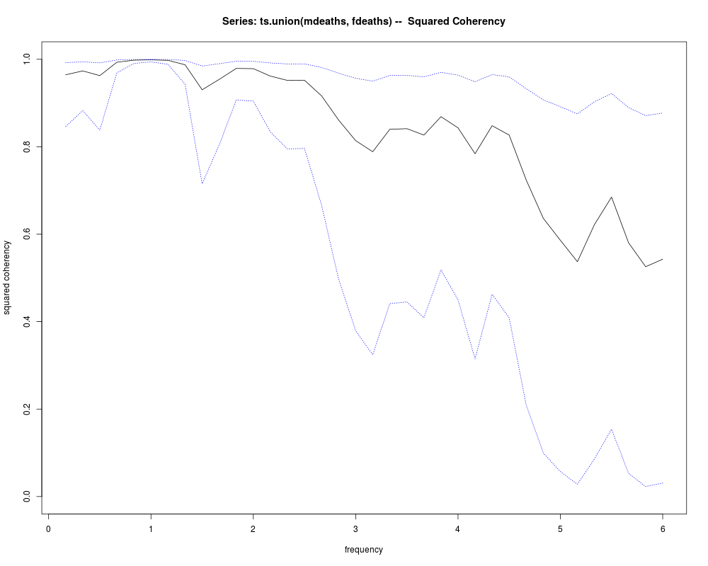
# plots marginal spectra: now plot coherency and phase
plot(mfdeaths.spc, plot.type = "coherency")
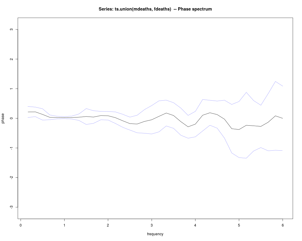
plot(mfdeaths.spc, plot.type = "phase")
## now impose a lack of alignment
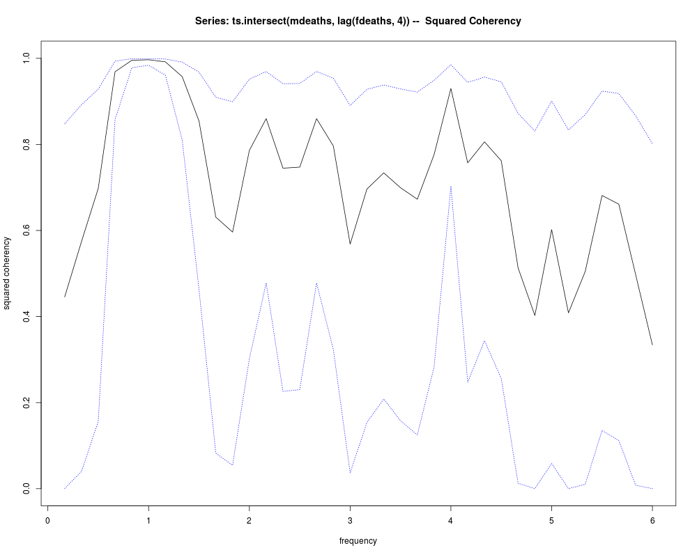
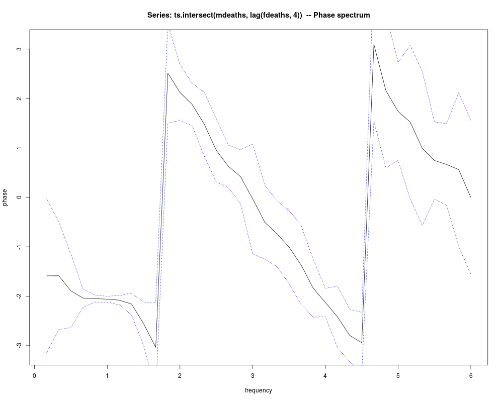
mfdeaths.spc <- spec.pgram(ts.intersect(mdeaths, lag(fdeaths, 4)),
spans = c(3,3), plot = FALSE)
plot(mfdeaths.spc, plot.type = "coherency")
plot(mfdeaths.spc, plot.type = "phase")
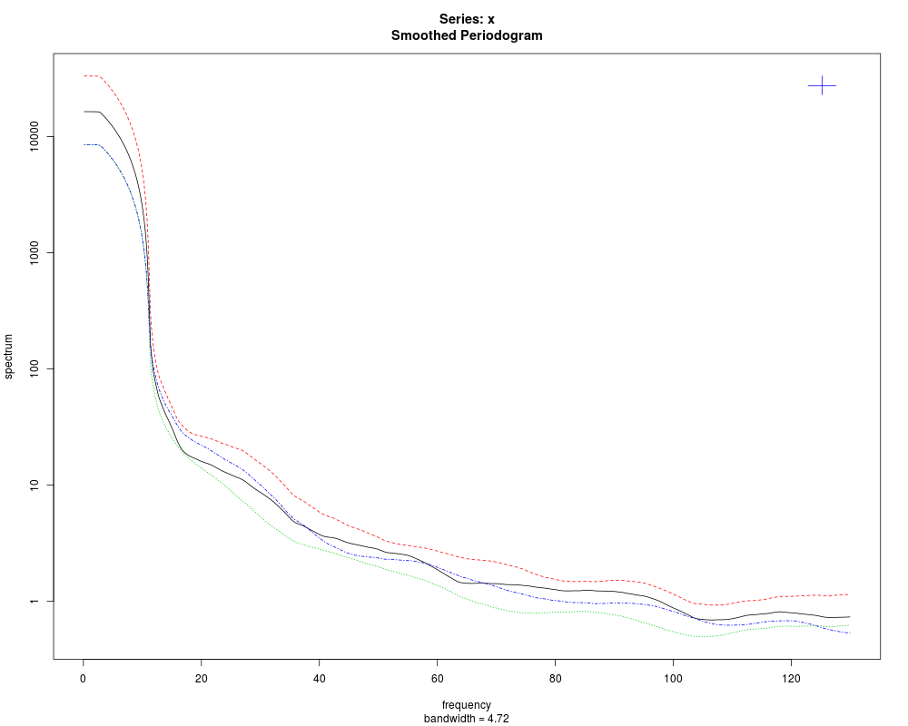
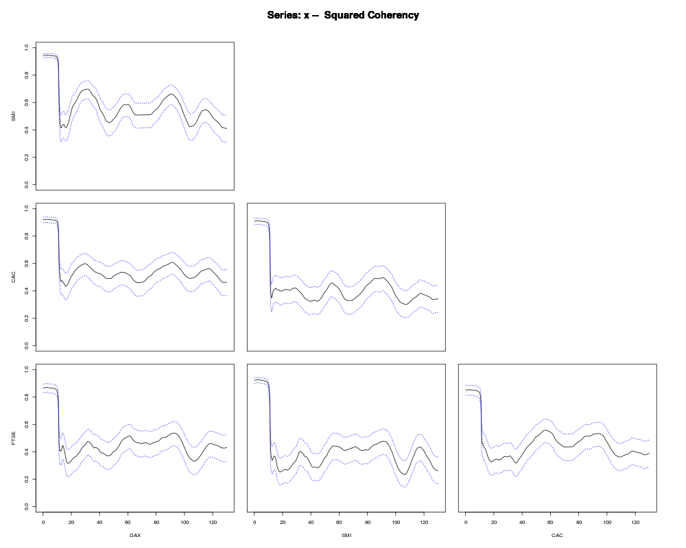
stocks.spc <- spectrum(EuStockMarkets, kernel("daniell", c(30,50)),
plot = FALSE)
plot(stocks.spc, plot.type = "marginal") # the default type
plot(stocks.spc, plot.type = "coherency")
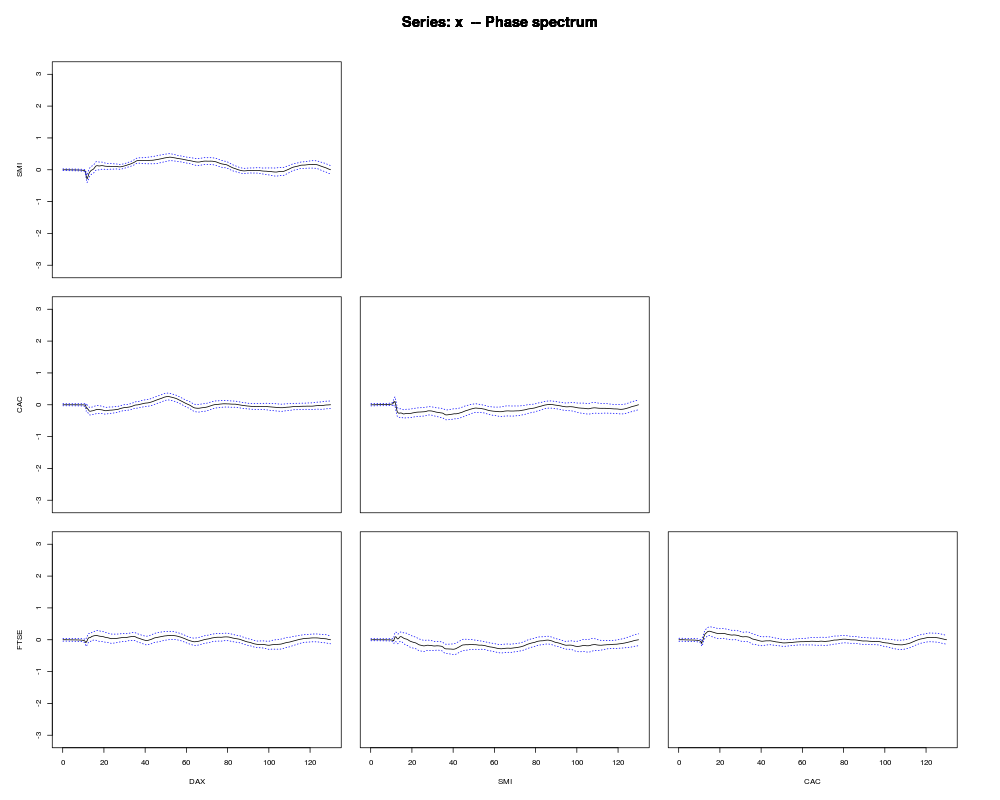
plot(stocks.spc, plot.type = "phase")
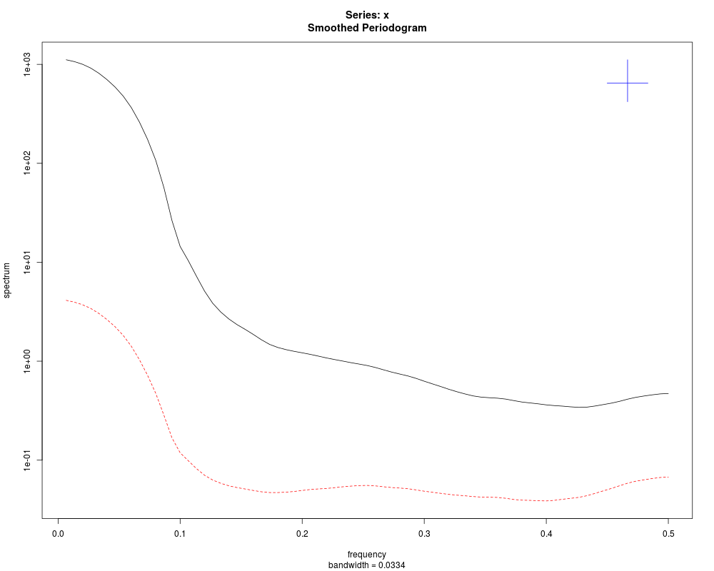
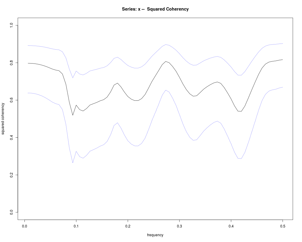
sales.spc <- spectrum(ts.union(BJsales, BJsales.lead),
kernel("modified.daniell", c(5,7)))
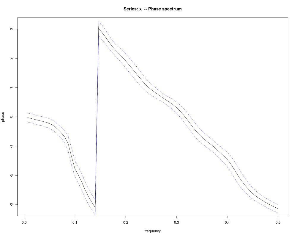
plot(sales.spc, plot.type = "coherency")
plot(sales.spc, plot.type = "phase")
Results
R version 3.3.1 (2016-06-21) -- "Bug in Your Hair"
Copyright (C) 2016 The R Foundation for Statistical Computing
Platform: x86_64-pc-linux-gnu (64-bit)

R is free software and comes with ABSOLUTELY NO WARRANTY.
You are welcome to redistribute it under certain conditions.
Type 'license()' or 'licence()' for distribution details.

R is a collaborative project with many contributors.
Type 'contributors()' for more information and
'citation()' on how to cite R or R packages in publications.

Type 'demo()' for some demos, 'help()' for on-line help, or
'help.start()' for an HTML browser interface to help.
Type 'q()' to quit R.

> library(stats)
> png(filename="/home/ddbj/snapshot/RGM3/R_rel/result/stats/spec.pgram.Rd_%03d_medium.png", width=480, height=480)
> ### Name: spec.pgram
> ### Title: Estimate Spectral Density of a Time Series by a Smoothed
> ###   Periodogram
> ### Aliases: spec.pgram
> ### Keywords: ts
>
> ### ** Examples
>
> require(graphics)
>
> ## Examples from Venables & Ripley
> spectrum(ldeaths)
> spectrum(ldeaths, spans = c(3,5))
> spectrum(ldeaths, spans = c(5,7))
> spectrum(mdeaths, spans = c(3,3))
> spectrum(fdeaths, spans = c(3,3))
>
> ## bivariate example
> mfdeaths.spc <- spec.pgram(ts.union(mdeaths, fdeaths), spans = c(3,3))
> # plots marginal spectra: now plot coherency and phase
> plot(mfdeaths.spc, plot.type = "coherency")
> plot(mfdeaths.spc, plot.type = "phase")
>
> ## now impose a lack of alignment
> mfdeaths.spc <- spec.pgram(ts.intersect(mdeaths, lag(fdeaths, 4)),
+    spans = c(3,3), plot = FALSE)
> plot(mfdeaths.spc, plot.type = "coherency")
> plot(mfdeaths.spc, plot.type = "phase")
>
> stocks.spc <- spectrum(EuStockMarkets, kernel("daniell", c(30,50)),
+                        plot = FALSE)
> plot(stocks.spc, plot.type = "marginal") # the default type
> plot(stocks.spc, plot.type = "coherency")
> plot(stocks.spc, plot.type = "phase")
>
> sales.spc <- spectrum(ts.union(BJsales, BJsales.lead),
+                       kernel("modified.daniell", c(5,7)))
> plot(sales.spc, plot.type = "coherency")
> plot(sales.spc, plot.type = "phase")
>
>
>
>
>
> dev.off()
null device
          1
>
|