R Graphical Manual

Browse All

Last data update: 2014.03.03

R: Maximum Likelihood Estimation

mle	R Documentation

Maximum Likelihood Estimation

Description

Estimate parameters by the method of maximum likelihood.

Usage

mle(minuslogl, start = formals(minuslogl), method = "BFGS",
    fixed = list(), nobs, ...)

Arguments

`minuslogl`	Function to calculate negative log-likelihood.
`start`	Named list. Initial values for optimizer.
`method`	Optimization method to use. See `optim`.
`fixed`	Named list. Parameter values to keep fixed during optimization.
`nobs`	optional integer: the number of observations, to be used for e.g. computing `BIC`.
`...`	Further arguments to pass to `optim`.

Details

The optim optimizer is used to find the minimum of the negative log-likelihood. An approximate covariance matrix for the parameters is obtained by inverting the Hessian matrix at the optimum.

Value

An object of class mle-class.

Note

Be careful to note that the argument is -log L (not -2 log L). It is for the user to ensure that the likelihood is correct, and that asymptotic likelihood inference is valid.

Examples

## Avoid printing to unwarranted accuracy
od <- options(digits = 5)
x <- 0:10
y <- c(26, 17, 13, 12, 20, 5, 9, 8, 5, 4, 8)

## Easy one-dimensional MLE:
nLL <- function(lambda) -sum(stats::dpois(y, lambda, log = TRUE))
fit0 <- mle(nLL, start = list(lambda = 5), nobs = NROW(y))
# For 1D, this is preferable:
fit1 <- mle(nLL, start = list(lambda = 5), nobs = NROW(y),
            method = "Brent", lower = 1, upper = 20)
stopifnot(nobs(fit0) == length(y))

## This needs a constrained parameter space: most methods will accept NA
ll <- function(ymax = 15, xhalf = 6) {
    if(ymax > 0 && xhalf > 0)
      -sum(stats::dpois(y, lambda = ymax/(1+x/xhalf), log = TRUE))
    else NA
}
(fit <- mle(ll, nobs = length(y)))
mle(ll, fixed = list(xhalf = 6))
## alternative using bounds on optimization
ll2 <- function(ymax = 15, xhalf = 6)
    -sum(stats::dpois(y, lambda = ymax/(1+x/xhalf), log = TRUE))
mle(ll2, method = "L-BFGS-B", lower = rep(0, 2))

AIC(fit)
BIC(fit)

summary(fit)
logLik(fit)
vcov(fit)
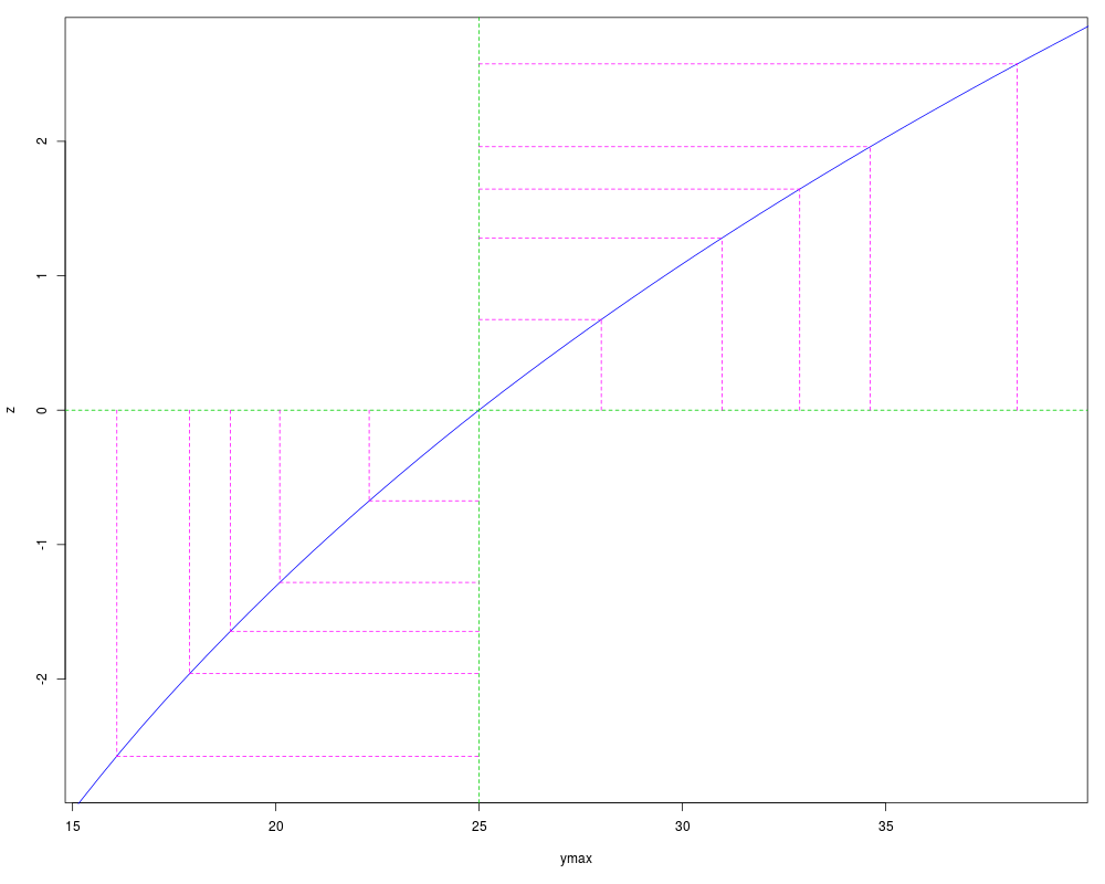
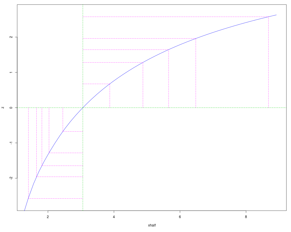
plot(profile(fit), absVal = FALSE)
confint(fit)

## Use bounded optimization
## The lower bounds are really > 0,
## but we use >=0 to stress-test profiling
(fit2 <- mle(ll, method = "L-BFGS-B", lower = c(0, 0)))
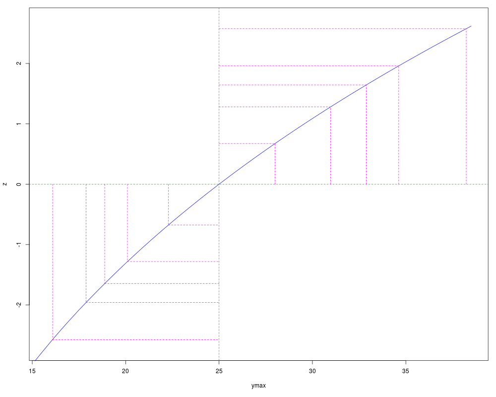
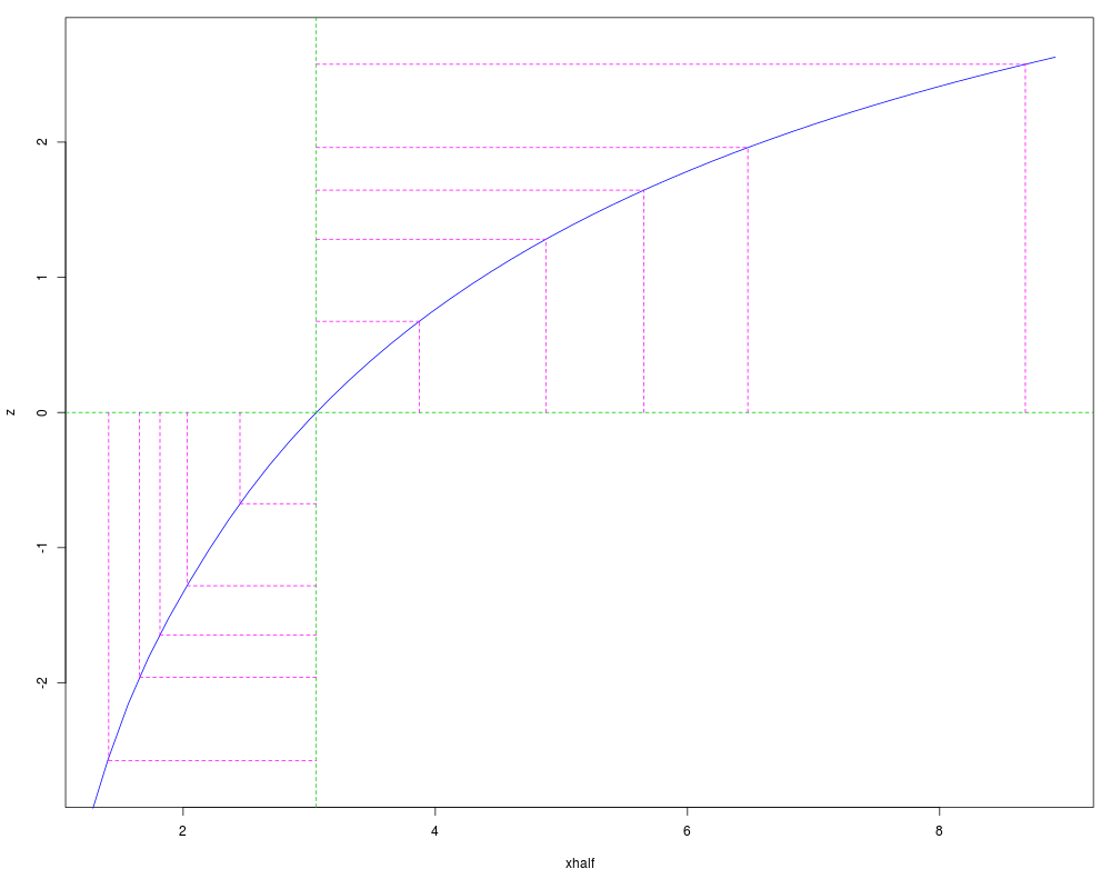
plot(profile(fit2), absVal = FALSE)

## a better parametrization:
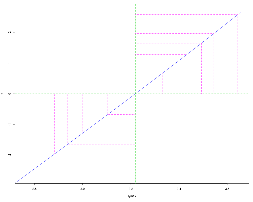
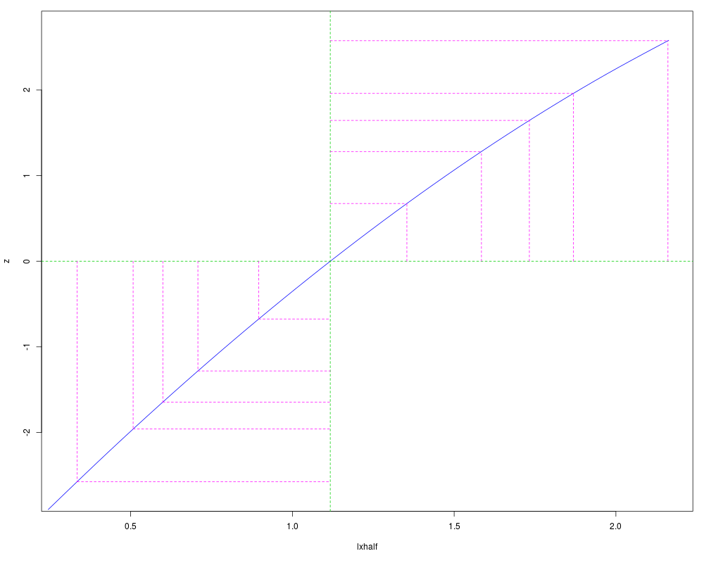
ll3 <- function(lymax = log(15), lxhalf = log(6))
    -sum(stats::dpois(y, lambda = exp(lymax)/(1+x/exp(lxhalf)), log = TRUE))
(fit3 <- mle(ll3))
plot(profile(fit3), absVal = FALSE)
exp(confint(fit3))

options(od)

Results


R version 3.3.1 (2016-06-21) -- "Bug in Your Hair"
Copyright (C) 2016 The R Foundation for Statistical Computing
Platform: x86_64-pc-linux-gnu (64-bit)

R is free software and comes with ABSOLUTELY NO WARRANTY.
You are welcome to redistribute it under certain conditions.
Type 'license()' or 'licence()' for distribution details.

R is a collaborative project with many contributors.
Type 'contributors()' for more information and
'citation()' on how to cite R or R packages in publications.

Type 'demo()' for some demos, 'help()' for on-line help, or
'help.start()' for an HTML browser interface to help.
Type 'q()' to quit R.

> library(stats4)
> png(filename="/home/ddbj/snapshot/RGM3/R_rel/result/stats4/mle.Rd_%03d_medium.png", width=480, height=480)
> ### Name: mle
> ### Title: Maximum Likelihood Estimation
> ### Aliases: mle
> ### Keywords: models
> 
> ### ** Examples
> 
> ## Avoid printing to unwarranted accuracy
> od <- options(digits = 5)
> x <- 0:10
> y <- c(26, 17, 13, 12, 20, 5, 9, 8, 5, 4, 8)
> 
> ## Easy one-dimensional MLE:
> nLL <- function(lambda) -sum(stats::dpois(y, lambda, log = TRUE))
> fit0 <- mle(nLL, start = list(lambda = 5), nobs = NROW(y))
> # For 1D, this is preferable:
> fit1 <- mle(nLL, start = list(lambda = 5), nobs = NROW(y),
+             method = "Brent", lower = 1, upper = 20)
> stopifnot(nobs(fit0) == length(y))
> 
> ## This needs a constrained parameter space: most methods will accept NA
> ll <- function(ymax = 15, xhalf = 6) {
+     if(ymax > 0 && xhalf > 0)
+       -sum(stats::dpois(y, lambda = ymax/(1+x/xhalf), log = TRUE))
+     else NA
+ }
> (fit <- mle(ll, nobs = length(y)))

Call:
mle(minuslogl = ll, nobs = length(y))

Coefficients:
   ymax   xhalf 
24.9931  3.0571 
> mle(ll, fixed = list(xhalf = 6))

Call:
mle(minuslogl = ll, fixed = list(xhalf = 6))

Coefficients:
  ymax  xhalf 
19.288  6.000 
> ## alternative using bounds on optimization
> ll2 <- function(ymax = 15, xhalf = 6)
+     -sum(stats::dpois(y, lambda = ymax/(1+x/xhalf), log = TRUE))
> mle(ll2, method = "L-BFGS-B", lower = rep(0, 2))

Call:
mle(minuslogl = ll2, method = "L-BFGS-B", lower = rep(0, 2))

Coefficients:
   ymax   xhalf 
24.9994  3.0558 
> 
> AIC(fit)
[1] 61.208
> BIC(fit)
[1] 62.004
> 
> summary(fit)
Maximum likelihood estimation

Call:
mle(minuslogl = ll, nobs = length(y))

Coefficients:
      Estimate Std. Error
ymax   24.9931     4.2244
xhalf   3.0571     1.0348

-2 log L: 57.208 
> logLik(fit)
'log Lik.' -28.604 (df=2)
> vcov(fit)
         ymax   xhalf
ymax  17.8459 -3.7206
xhalf -3.7206  1.0708
> plot(profile(fit), absVal = FALSE)
> confint(fit)
Profiling...
        2.5 %  97.5 %
ymax  17.8845 34.6194
xhalf  1.6616  6.4792
> 
> ## Use bounded optimization
> ## The lower bounds are really > 0,
> ## but we use >=0 to stress-test profiling
> (fit2 <- mle(ll, method = "L-BFGS-B", lower = c(0, 0)))

Call:
mle(minuslogl = ll, method = "L-BFGS-B", lower = c(0, 0))

Coefficients:
   ymax   xhalf 
24.9994  3.0558 
> plot(profile(fit2), absVal = FALSE)
> 
> ## a better parametrization:
> ll3 <- function(lymax = log(15), lxhalf = log(6))
+     -sum(stats::dpois(y, lambda = exp(lymax)/(1+x/exp(lxhalf)), log = TRUE))
> (fit3 <- mle(ll3))

Call:
mle(minuslogl = ll3)

Coefficients:
 lymax lxhalf 
3.2189 1.1170 
> plot(profile(fit3), absVal = FALSE)
> exp(confint(fit3))
Profiling...
         2.5 %  97.5 %
lymax  17.8815 34.6186
lxhalf  1.6615  6.4794
> 
> options(od)
> 
> 
> 
> 
> 
> dev.off()
null device 
          1 
>