Supported by Dr. Osamu Ogasawara and  . . |
|
Last data update: 2014.03.03 |
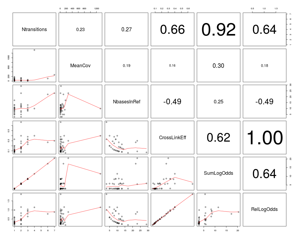
Pairs plot visualization of clusters statisticsDescriptionGraphical representation of cluster statistics, featuring pairwise correlations in the upper panel. UsageplotStatistics(clusters, corMethod = 'spearman', lower = panel.smooth, ...) Arguments
Valuecalled for its effect Author(s)Federico Comoglio See Also
Examples
require(BSgenome.Hsapiens.UCSC.hg19)

data( model, package = "wavClusteR" )

filename <- system.file( "extdata", "example.bam", package = "wavClusteR" )
example <- readSortedBam( filename = filename )
countTable <- getAllSub( example, minCov = 10, cores = 1 )
highConfSub <- getHighConfSub( countTable, supportStart = 0.2, supportEnd = 0.7, substitution = "TC" )
coverage <- coverage( example )
clusters <- getClusters( highConfSub = highConfSub,
                         coverage = coverage,
                         sortedBam = example,
	                 method = 'mrn',
	                 cores = 1,
	                 threshold = 2 )

fclusters <- filterClusters( clusters = clusters,
		             highConfSub = highConfSub,
        		     coverage = coverage,
			     model = model,
			     genome = Hsapiens,
		             refBase = 'T',
		             minWidth = 12 )
plotStatistics( clusters = fclusters )
Results
R version 3.3.1 (2016-06-21) -- "Bug in Your Hair"
Copyright (C) 2016 The R Foundation for Statistical Computing
Platform: x86_64-pc-linux-gnu (64-bit)

R is free software and comes with ABSOLUTELY NO WARRANTY.
You are welcome to redistribute it under certain conditions.
Type 'license()' or 'licence()' for distribution details.

R is a collaborative project with many contributors.
Type 'contributors()' for more information and
'citation()' on how to cite R or R packages in publications.

Type 'demo()' for some demos, 'help()' for on-line help, or
'help.start()' for an HTML browser interface to help.
Type 'q()' to quit R.

> library(wavClusteR)
Loading required package: GenomicRanges
Loading required package: BiocGenerics
Loading required package: parallel

Attaching package: 'BiocGenerics'

The following objects are masked from 'package:parallel':

    clusterApply, clusterApplyLB, clusterCall, clusterEvalQ,
    clusterExport, clusterMap, parApply, parCapply, parLapply,
    parLapplyLB, parRapply, parSapply, parSapplyLB

The following objects are masked from 'package:stats':

    IQR, mad, xtabs

The following objects are masked from 'package:base':

    Filter, Find, Map, Position, Reduce, anyDuplicated, append,
    as.data.frame, cbind, colnames, do.call, duplicated, eval, evalq,
    get, grep, grepl, intersect, is.unsorted, lapply, lengths, mapply,
    match, mget, order, paste, pmax, pmax.int, pmin, pmin.int, rank,
    rbind, rownames, sapply, setdiff, sort, table, tapply, union,
    unique, unsplit

Loading required package: S4Vectors
Loading required package: stats4

Attaching package: 'S4Vectors'

The following objects are masked from 'package:base':

    colMeans, colSums, expand.grid, rowMeans, rowSums

Loading required package: IRanges
Loading required package: GenomeInfoDb
Loading required package: Rsamtools
Loading required package: Biostrings
Loading required package: XVector
> png(filename="/home/ddbj/snapshot/RGM3/R_BC/result/wavClusteR/plotStatistics.Rd_%03d_medium.png", width=480, height=480)
> ### Name: plotStatistics
> ### Title: Pairs plot visualization of clusters statistics
> ### Aliases: plotStatistics
> ### Keywords: graphics postprocessing
>
> ### ** Examples
>
>
> require(BSgenome.Hsapiens.UCSC.hg19)
Loading required package: BSgenome.Hsapiens.UCSC.hg19
Loading required package: BSgenome
Loading required package: rtracklayer
>
> data( model, package = "wavClusteR" )
>
> filename <- system.file( "extdata", "example.bam", package = "wavClusteR" )
> example <- readSortedBam( filename = filename )
> countTable <- getAllSub( example, minCov = 10, cores = 1 )
Loading required package: doMC
Loading required package: foreach
Loading required package: iterators
Considering substitutions, n = 497, processing in 1 chunks
   chunk #: 1
   considering the + strand
Computing local coverage at substitutions...
   considering the - strand
Computing local coverage at substitutions...
> highConfSub <- getHighConfSub( countTable, supportStart = 0.2, supportEnd = 0.7, substitution = "TC" )
> coverage <- coverage( example )
> clusters <- getClusters( highConfSub = highConfSub,
+                          coverage = coverage,
+                          sortedBam = example,
+ 	                 method = 'mrn',
+ 	                 cores = 1,
+ 	                 threshold = 2 )
Computing start/end read positions
Number of chromosomes exhibiting high confidence transitions: 1
...Processing = chrX
>
> fclusters <- filterClusters( clusters = clusters,
+ 		             highConfSub = highConfSub,
+         		     coverage = coverage,
+ 			     model = model,
+ 			     genome = Hsapiens,
+ 		             refBase = 'T',
+ 		             minWidth = 12 )
Computing log odds...
Refining cluster sizes...
Combining clusters...
Quantifying transitions within clusters...
Computing statistics...
   |                                                                               |==                                                                    |   3%   |                                                                               |====                                                                  |   5%   |                                                                               |=====                                                                 |   8%   |                                                                               |=======                                                               |  10%   |                                                                               |=========                                                             |  13%   |                                                                               |===========                                                           |  15%   |                                                                               |=============                                                         |  18%   |                                                                               |==============                                                        |  21%   |                                                                               |================                                                      |  23%   |                                                                               |==================                                                    |  26%   |                                                                               |====================                                                  |  28%   |                                                                               |======================                                                |  31%   |                                                                               |=======================                                               |  33%   |                                                                               |=========================                                             |  36%   |                                                                               |===========================                                           |  38%   |                                                                               |=============================                                         |  41%   |                                                                               |===============================                                       |  44%   |                                                                               |================================                                      |  46%   |                                                                               |==================================                                    |  49%   |                                                                               |====================================                                  |  51%   |                                                                               |======================================                                |  54%   |                                                                               |=======================================                               |  56%   |                                                                               |=========================================                             |  59%   |                                                                               |===========================================                           |  62%   |                                                                               |=============================================                         |  64%   |                                                                               |===============================================                       |  67%   |                                                                               |================================================                      |  69%   |                                                                               |==================================================                    |  72%   |                                                                               |====================================================                  |  74%   |                                                                               |======================================================                |  77%   |                                                                               |========================================================              |  79%   |                                                                               |=========================================================             |  82%   |                                                                               |===========================================================           |  85%   |                                                                               |=============================================================         |  87%   |                                                                               |===============================================================       |  90%   |                                                                               |=================================================================     |  92%   |                                                                               |==================================================================    |  95%   |                                                                               |====================================================================  |  97%   |                                                                               |======================================================================| 100%
Consolidating results...
> plotStatistics( clusters = fclusters )
>
>
>
>
>
>
> dev.off()
null device
          1
>
|
Created & Maintained by Osamu Ogasawara (osamu.ogasawara@gmail.com) and 