Supported by Dr. Osamu Ogasawara and  . . |
|
Last data update: 2014.03.03 |
Data and Examples from Franses (1998)DescriptionThis manual page collects a list of examples from the book. Some solutions might not be exact and the list is certainly not complete. If you have suggestions for improvement (preferably in the form of code), please contact the package maintainer. ReferencesFranses, P.H. (1998). Time Series Models for Business and Economic Forecasting. Cambridge, UK: Cambridge University Press. URL http://www.few.eur.nl/few/people/franses/research/book2.htm. See Also
Examples
###########################
## Convenience functions ##
###########################
## EACF tables (Franses 1998, p. 99)
ctrafo <- function(x) residuals(lm(x ~ factor(cycle(x))))
ddiff <- function(x) diff(diff(x, frequency(x)), 1)
eacf <- function(y, lag = 12) {
stopifnot(all(lag > 0))
if(length(lag) < 2) lag <- 1:lag
rval <- sapply(
list(y = y, dy = diff(y), cdy = ctrafo(diff(y)),
Dy = diff(y, frequency(y)), dDy = ddiff(y)),
function(x) acf(x, plot = FALSE, lag.max = max(lag))$acf[lag + 1])
rownames(rval) <- lag
return(rval)
}
#######################################
## Index of US industrial production ##
#######################################
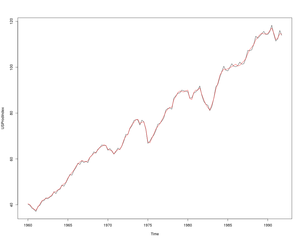
data("USProdIndex", package = "AER")
plot(USProdIndex, plot.type = "single", col = 1:2)
## Franses (1998), Table 5.1
round(eacf(log(USProdIndex[,1])), digits = 3)
## Franses (1998), Equation 5.6: Unrestricted airline model
## (Franses: ma1 = 0.388 (0.063), ma4 = -0.739 (0.060), ma5 = -0.452 (0.069))
arima(log(USProdIndex[,1]), c(0, 1, 5), c(0, 1, 0), fixed = c(NA, 0, 0, NA, NA))
###########################################
## Consumption of non-durables in the UK ##
###########################################
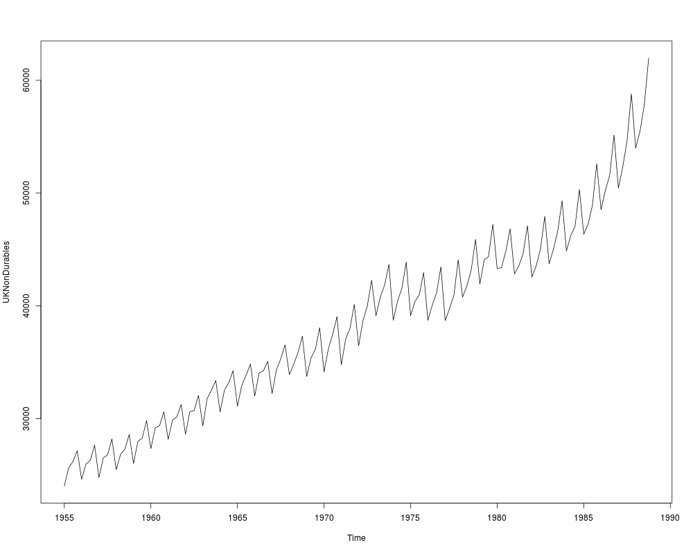
data("UKNonDurables", package = "AER")
plot(UKNonDurables)
## Franses (1998), Table 5.2
round(eacf(log(UKNonDurables)), digits = 3)
## Franses (1998), Equation 5.51
## (Franses: sma1 = -0.632 (0.069))
arima(log(UKNonDurables), c(0, 1, 0), c(0, 1, 1))
##############################
## Dutch retail sales index ##
##############################
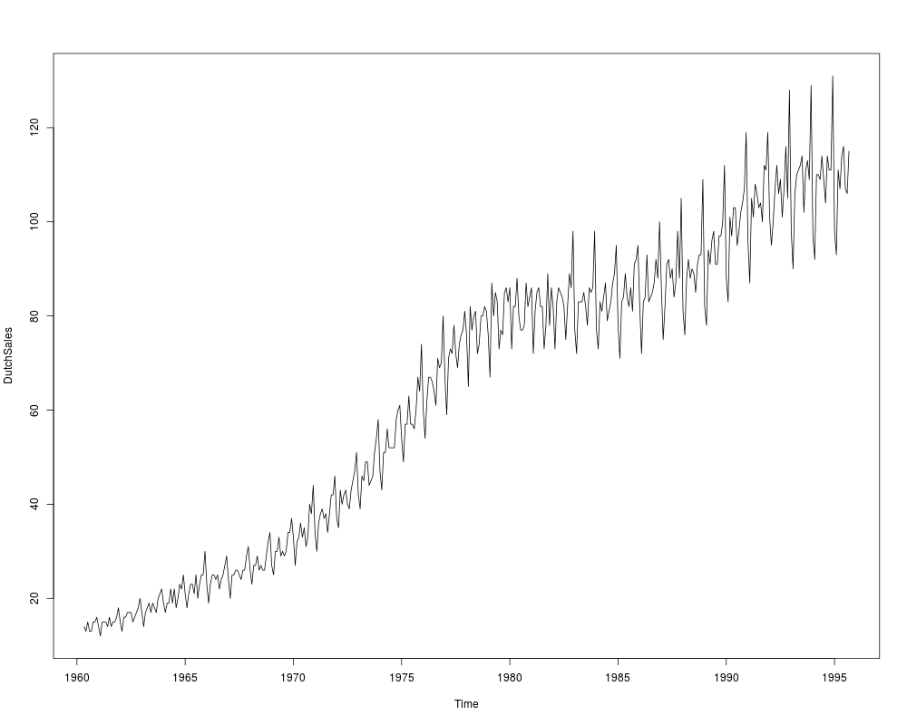
data("DutchSales", package = "AER")
plot(DutchSales)
## Franses (1998), Table 5.3
round(eacf(log(DutchSales), lag = c(1:18, 24, 36)), digits = 3)
###########################################
## TV and radio advertising expenditures ##
###########################################
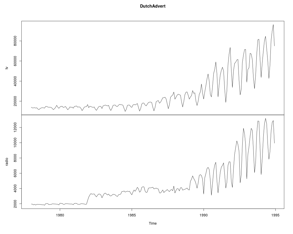
data("DutchAdvert", package = "AER")
plot(DutchAdvert)
## Franses (1998), Table 5.4
round(eacf(log(DutchAdvert[,"tv"]), lag = c(1:19, 26, 39)), digits = 3)
Results
R version 3.3.1 (2016-06-21) -- "Bug in Your Hair"
Copyright (C) 2016 The R Foundation for Statistical Computing
Platform: x86_64-pc-linux-gnu (64-bit)

R is free software and comes with ABSOLUTELY NO WARRANTY.
You are welcome to redistribute it under certain conditions.
Type 'license()' or 'licence()' for distribution details.

R is a collaborative project with many contributors.
Type 'contributors()' for more information and
'citation()' on how to cite R or R packages in publications.

Type 'demo()' for some demos, 'help()' for on-line help, or
'help.start()' for an HTML browser interface to help.
Type 'q()' to quit R.

> library(AER)
Loading required package: car
Loading required package: lmtest
Loading required package: zoo

Attaching package: 'zoo'

The following objects are masked from 'package:base':

    as.Date, as.Date.numeric

Loading required package: sandwich
Loading required package: survival
> png(filename="/home/ddbj/snapshot/RGM3/R_CC/result/AER/Franses1998.Rd_%03d_medium.png", width=480, height=480)
> ### Name: Franses1998
> ### Title: Data and Examples from Franses (1998)
> ### Aliases: Franses1998
> ### Keywords: datasets
>
> ### ** Examples
>
> ###########################
> ## Convenience functions ##
> ###########################
>
> ## EACF tables (Franses 1998, p. 99)
> ctrafo <- function(x) residuals(lm(x ~ factor(cycle(x))))
> ddiff <- function(x) diff(diff(x, frequency(x)), 1)
> eacf <- function(y, lag = 12) {
+   stopifnot(all(lag > 0))
+   if(length(lag) < 2) lag <- 1:lag
+   rval <- sapply(
+     list(y = y, dy = diff(y), cdy = ctrafo(diff(y)),
+          Dy = diff(y, frequency(y)), dDy = ddiff(y)),
+     function(x) acf(x, plot = FALSE, lag.max = max(lag))$acf[lag + 1])
+   rownames(rval) <- lag
+   return(rval)
+ }
>
> #######################################
> ## Index of US industrial production ##
> #######################################
>
> data("USProdIndex", package = "AER")
> plot(USProdIndex, plot.type = "single", col = 1:2)
>
> ## Franses (1998), Table 5.1
> round(eacf(log(USProdIndex[,1])), digits = 3)
       y     dy    cdy     Dy    dDy
1  0.975  0.162  0.242  0.851  0.535
2  0.947  0.140  0.196  0.586  0.162
3  0.918 -0.110 -0.061  0.295 -0.051
4  0.888  0.300  0.205  0.036 -0.328
5  0.853 -0.268 -0.264 -0.126 -0.296
6  0.821 -0.046 -0.032 -0.220 -0.190
7  0.789 -0.249 -0.224 -0.274 -0.165
8  0.761  0.120  0.008 -0.296 -0.204
9  0.732 -0.257 -0.253 -0.262 -0.066
10 0.705  0.015  0.044 -0.207  0.080
11 0.676 -0.198 -0.165 -0.172  0.025
12 0.649  0.199  0.099 -0.138  0.018
>
> ## Franses (1998), Equation 5.6: Unrestricted airline model
> ## (Franses: ma1 = 0.388 (0.063), ma4 = -0.739 (0.060), ma5 = -0.452 (0.069))
> arima(log(USProdIndex[,1]), c(0, 1, 5), c(0, 1, 0), fixed = c(NA, 0, 0, NA, NA))

Call:
arima(x = log(USProdIndex[, 1]), order = c(0, 1, 5), seasonal = c(0, 1, 0),
    fixed = c(NA, 0, 0, NA, NA))

Coefficients:
         ma1  ma2  ma3      ma4      ma5
      0.4603    0    0  -0.7731  -0.5313
s.e.  0.0707    0    0   0.0626   0.0713

sigma^2 estimated as 0.0003366:  log likelihood = 314.84,  aic = -621.69
>
> ###########################################
> ## Consumption of non-durables in the UK ##
> ###########################################
>
> data("UKNonDurables", package = "AER")
> plot(UKNonDurables)
>
> ## Franses (1998), Table 5.2
> round(eacf(log(UKNonDurables)), digits = 3)
       y     dy    cdy     Dy    dDy
1  0.928 -0.463 -0.074  0.779 -0.164
2  0.900 -0.014 -0.359  0.625  0.050
3  0.876 -0.481 -0.034  0.449  0.048
4  0.891  0.947  0.554  0.248 -0.444
5  0.823 -0.438  0.023  0.238  0.236
6  0.795 -0.014 -0.390  0.130 -0.118
7  0.771 -0.471 -0.045  0.082  0.115
8  0.788  0.910  0.491 -0.014  0.023
9  0.723 -0.421 -0.081 -0.125 -0.251
10 0.697 -0.014 -0.328 -0.133  0.122
11 0.674 -0.464 -0.148 -0.196 -0.131
12 0.691  0.877  0.414 -0.196 -0.001
>
> ## Franses (1998), Equation 5.51
> ## (Franses: sma1 = -0.632 (0.069))
> arima(log(UKNonDurables), c(0, 1, 0), c(0, 1, 1))

Call:
arima(x = log(UKNonDurables), order = c(0, 1, 0), seasonal = c(0, 1, 1))

Coefficients:
         sma1
      -0.6095
s.e.   0.0711

sigma^2 estimated as 0.0001234:  log likelihood = 402.71,  aic = -801.42
>
> ##############################
> ## Dutch retail sales index ##
> ##############################
>
> data("DutchSales", package = "AER")
> plot(DutchSales)
>
> ## Franses (1998), Table 5.3
> round(eacf(log(DutchSales), lag = c(1:18, 24, 36)), digits = 3)
       y     dy    cdy    Dy    dDy
1  0.980 -0.264 -0.556 0.456 -0.532
2  0.967 -0.238 -0.024 0.490 -0.121
3  0.961 -0.004  0.221 0.654  0.307
4  0.954 -0.256 -0.180 0.486 -0.200
5  0.954  0.163  0.010 0.534 -0.011
6  0.950  0.236  0.160 0.593  0.148
7  0.940  0.093 -0.150 0.492 -0.093
8  0.929 -0.195 -0.025 0.492 -0.106
9  0.922 -0.004  0.223 0.607  0.268
10 0.912 -0.306 -0.256 0.431 -0.276
11 0.913 -0.098 -0.035 0.556  0.228
12 0.916  0.816  0.453 0.432 -0.061
13 0.897 -0.248 -0.497 0.375 -0.290
14 0.885 -0.113  0.344 0.633  0.408
15 0.877 -0.112 -0.125 0.446 -0.119
16 0.870 -0.238 -0.109 0.392 -0.189
17 0.870  0.218  0.176 0.540  0.240
18 0.865  0.181 -0.008 0.429 -0.045
24 0.827  0.656 -0.007 0.300 -0.308
36 0.738  0.593 -0.125 0.210 -0.312
>
> ###########################################
> ## TV and radio advertising expenditures ##
> ###########################################
>
> data("DutchAdvert", package = "AER")
> plot(DutchAdvert)
>
> ## Franses (1998), Table 5.4
> round(eacf(log(DutchAdvert[,"tv"]), lag = c(1:19, 26, 39)), digits = 3)
       y     dy    cdy    Dy    dDy
1  0.933  0.215  0.039 0.663 -0.301
2  0.836 -0.352 -0.255 0.529 -0.111
3  0.781 -0.418 -0.316 0.471 -0.083
4  0.774 -0.351 -0.301 0.466  0.044
5  0.813 -0.013 -0.020 0.431  0.001
6  0.857  0.417  0.346 0.393 -0.003
7  0.848  0.438  0.409 0.357  0.036
8  0.786 -0.008  0.024 0.299  0.008
9  0.723 -0.348 -0.308 0.233 -0.031
10 0.700 -0.398 -0.288 0.191 -0.022
11 0.725 -0.324 -0.191 0.162  0.026
12 0.788  0.240  0.109 0.119  0.105
13 0.829  0.810  0.531 0.004 -0.412
14 0.773  0.265  0.183 0.172  0.312
15 0.683 -0.331 -0.210 0.125 -0.103
16 0.630 -0.370 -0.222 0.146  0.096
17 0.621 -0.334 -0.277 0.103  0.008
18 0.656 -0.025 -0.053 0.050 -0.187
19 0.699  0.383  0.274 0.127  0.003
26 0.672  0.728  0.399 0.111 -0.002
39 0.500  0.650  0.294 0.172  0.034
>
>
>
>
>
> dev.off()
null device
          1
>
|
Created & Maintained by Osamu Ogasawara (osamu.ogasawara@gmail.com) and 