Supported by Dr. Osamu Ogasawara and  . . |
|
Last data update: 2014.03.03 |
US General Social Survey 1974–2002DescriptionCross-section data for 9120 women taken from every fourth year of the US General Social Survey between 1974 and 2002 to investigate the determinants of fertility. Usagedata("GSS7402")
FormatA data frame containing 9120 observations on 10 variables.
DetailsThis subset of the US General Social Survey (GSS) for every fourth year between 1974 and 2002 has been selected by Winkelmann and Boes (2009) to investigate the determinants of fertility. To do so they typically restrict their empirical analysis to the women for which the completed fertility is (assumed to be) known, employing the common cutoff of 40 years. Both, the average number of children borne to a woman and the probability of being childless, are of interest. SourceOnline complements to Winkelmann and Boes (2009). http://www.econ.uzh.ch/faculty/groupwinkelmann/research/publications/microdata/datasets/kids.zip ReferencesWinkelmann, R., and Boes, S. (2009). Analysis of Microdata, 2nd ed. Berlin and Heidelberg: Springer-Verlag. See Also
Examples
## completed fertility subset
data("GSS7402", package = "AER")
gss40 <- subset(GSS7402, age >= 40)
## Chapter 1
## exploratory statistics
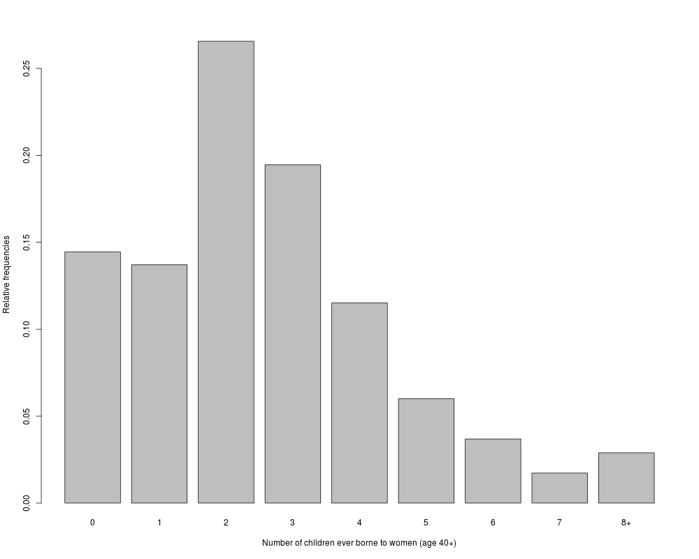
gss_kids <- prop.table(table(gss40$kids))
names(gss_kids)[9] <- "8+"
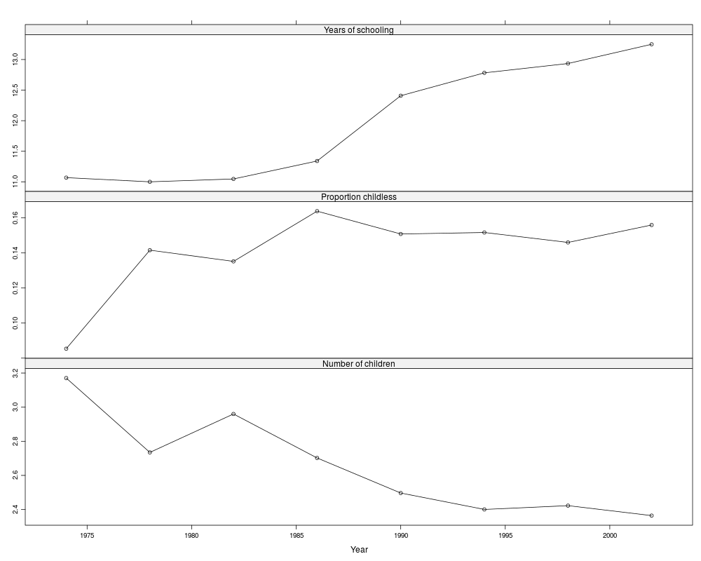
gss_zoo <- as.matrix(with(gss40, cbind(
tapply(kids, year, mean),
tapply(kids, year, function(x) mean(x <= 0)),
tapply(education, year, mean))))
colnames(gss_zoo) <- c("Number of children",
"Proportion childless", "Years of schooling")
gss_zoo <- zoo(gss_zoo, sort(unique(gss40$year)))
## visualizations instead of tables
barplot(gss_kids,
xlab = "Number of children ever borne to women (age 40+)",
ylab = "Relative frequencies")
library("lattice")
trellis.par.set(theme = canonical.theme(color = FALSE))
print(xyplot(gss_zoo[,3:1], type = "b", xlab = "Year"))
## Chapter 3, Example 3.14
## Table 3.1
gss40$nokids <- factor(gss40$kids <= 0, levels = c(FALSE, TRUE), labels = c("no", "yes"))
gss40$trend <- gss40$year - 1974
nokids_p1 <- glm(nokids ~ 1, data = gss40, family = binomial(link = "probit"))
nokids_p2 <- glm(nokids ~ trend, data = gss40, family = binomial(link = "probit"))
nokids_p3 <- glm(nokids ~ trend + education + ethnicity + siblings,
data = gss40, family = binomial(link = "probit"))
lrtest(nokids_p1, nokids_p2, nokids_p3)
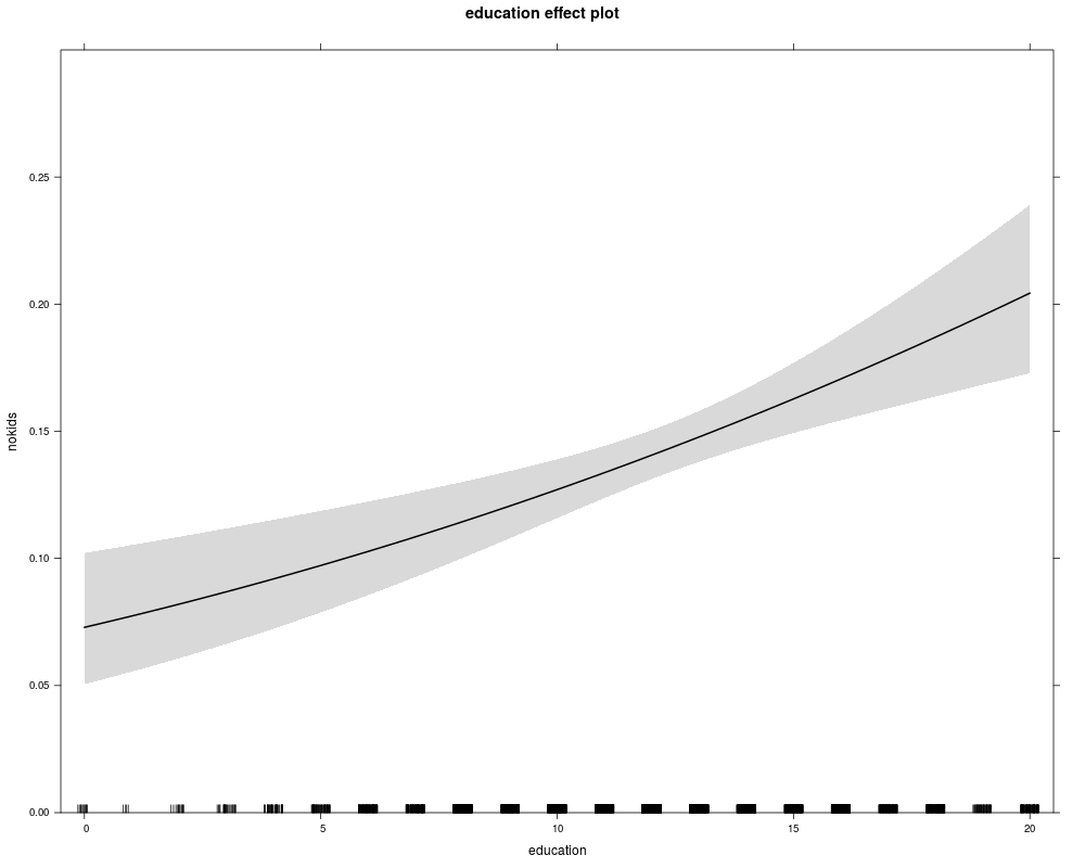
## Chapter 4, Figure 4.4
library("effects")
nokids_p3_ef <- effect("education", nokids_p3, xlevels = list(education = 0:20))
plot(nokids_p3_ef, rescale.axis = FALSE, ylim = c(0, 0.3))
## Chapter 8, Example 8.11
kids_pois <- glm(kids ~ education + trend + ethnicity + immigrant + lowincome16 + city16,
data = gss40, family = poisson)
library("MASS")
kids_nb <- glm.nb(kids ~ education + trend + ethnicity + immigrant + lowincome16 + city16,
data = gss40)
lrtest(kids_pois, kids_nb)
## More examples can be found in:
## help("WinkelmannBoes2009")
Results
R version 3.3.1 (2016-06-21) -- "Bug in Your Hair"
Copyright (C) 2016 The R Foundation for Statistical Computing
Platform: x86_64-pc-linux-gnu (64-bit)

R is free software and comes with ABSOLUTELY NO WARRANTY.
You are welcome to redistribute it under certain conditions.
Type 'license()' or 'licence()' for distribution details.

R is a collaborative project with many contributors.
Type 'contributors()' for more information and
'citation()' on how to cite R or R packages in publications.

Type 'demo()' for some demos, 'help()' for on-line help, or
'help.start()' for an HTML browser interface to help.
Type 'q()' to quit R.

> library(AER)
Loading required package: car
Loading required package: lmtest
Loading required package: zoo

Attaching package: 'zoo'

The following objects are masked from 'package:base':

    as.Date, as.Date.numeric

Loading required package: sandwich
Loading required package: survival
> png(filename="/home/ddbj/snapshot/RGM3/R_CC/result/AER/GSS7402.Rd_%03d_medium.png", width=480, height=480)
> ### Name: GSS7402
> ### Title: US General Social Survey 1974-2002
> ### Aliases: GSS7402
> ### Keywords: datasets
>
> ### ** Examples
>
> ## completed fertility subset
> data("GSS7402", package = "AER")
> gss40 <- subset(GSS7402, age >= 40)
>
> ## Chapter 1
> ## exploratory statistics
> gss_kids <- prop.table(table(gss40$kids))
> names(gss_kids)[9] <- "8+"
>
> gss_zoo <- as.matrix(with(gss40, cbind(
+   tapply(kids, year, mean),
+   tapply(kids, year, function(x) mean(x <= 0)),
+   tapply(education, year, mean))))
> colnames(gss_zoo) <- c("Number of children",
+   "Proportion childless", "Years of schooling")
> gss_zoo <- zoo(gss_zoo, sort(unique(gss40$year)))
>
> ## visualizations instead of tables
> barplot(gss_kids,
+   xlab = "Number of children ever borne to women (age 40+)",
+   ylab = "Relative frequencies")
>
> library("lattice")
> trellis.par.set(theme = canonical.theme(color = FALSE))
> print(xyplot(gss_zoo[,3:1], type = "b", xlab = "Year"))
>
>
> ## Chapter 3, Example 3.14
> ## Table 3.1
> gss40$nokids <- factor(gss40$kids <= 0, levels = c(FALSE, TRUE), labels = c("no", "yes"))
> gss40$trend <- gss40$year - 1974
> nokids_p1 <- glm(nokids ~ 1, data = gss40, family = binomial(link = "probit"))
> nokids_p2 <- glm(nokids ~ trend, data = gss40, family = binomial(link = "probit"))
> nokids_p3 <- glm(nokids ~ trend + education + ethnicity + siblings,
+   data = gss40, family = binomial(link = "probit"))
> lrtest(nokids_p1, nokids_p2, nokids_p3)
Likelihood ratio test

Model 1: nokids ~ 1
Model 2: nokids ~ trend
Model 3: nokids ~ trend + education + ethnicity + siblings
  #Df  LogLik Df   Chisq Pr(>Chisq)
1   1 -2126.9
2   2 -2123.6  1  6.5677    0.01038 *
3   5 -2107.1  3 32.9906  3.235e-07 ***
---
Signif. codes:  0 '***' 0.001 '**' 0.01 '*' 0.05 '.' 0.1 ' ' 1
>
>
> ## Chapter 4, Figure 4.4
> library("effects")

Attaching package: 'effects'

The following object is masked from 'package:car':

    Prestige

> nokids_p3_ef <- effect("education", nokids_p3, xlevels = list(education = 0:20))
> plot(nokids_p3_ef, rescale.axis = FALSE, ylim = c(0, 0.3))
NOTE: the rescale.axis argument is deprecated; use type instead
>
>
> ## Chapter 8, Example 8.11
> kids_pois <- glm(kids ~ education + trend + ethnicity + immigrant + lowincome16 + city16,
+   data = gss40, family = poisson)
> library("MASS")
> kids_nb <- glm.nb(kids ~ education + trend + ethnicity + immigrant + lowincome16 + city16,
+   data = gss40)
> lrtest(kids_pois, kids_nb)
Likelihood ratio test

Model 1: kids ~ education + trend + ethnicity + immigrant + lowincome16 +
    city16
Model 2: kids ~ education + trend + ethnicity + immigrant + lowincome16 +
    city16
  #Df LogLik Df  Chisq Pr(>Chisq)
1   7 -10117
2   8 -10014  1 205.17  < 2.2e-16 ***
---
Signif. codes:  0 '***' 0.001 '**' 0.01 '*' 0.05 '.' 0.1 ' ' 1
>
>
> ## More examples can be found in:
> ## help("WinkelmannBoes2009")
>
>
>
>
>
> dev.off()
null device
          1
>
|