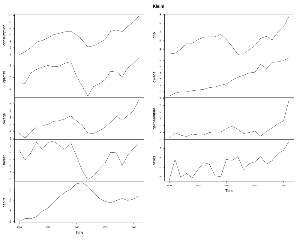
Klein Model I

Description

Klein's Model I for the US economy.

Usage

data("KleinI")

Format

An annual multiple time series from 1920 to 1941 with 9 variables.

consumption

Consumption.

cprofits

Corporate profits.

pwage

Private wage bill.

invest

Investment.

capital

Previous year's capital stock.

gnp

Gross national product.

gwage

Government wage bill.

gexpenditure

Government spending.

taxes

Taxes.

Source

Online complements to Greene (2003). Table F15.1.

http://pages.stern.nyu.edu/~wgreene/Text/tables/tablelist5.htm

References

Greene, W.H. (2003). Econometric Analysis, 5th edition. Upper Saddle River, NJ: Prentice Hall.

Klein, L. (1950). Economic Fluctuations in the United States, 1921–1941. New York: John Wiley.

Maddala, G.S. (1977). Econometrics. New York: McGraw-Hill.

See Also

Greene2003

Examples

data("KleinI", package = "AER")
plot(KleinI)

## Greene (2003), Tab. 15.3, OLS
library("dynlm")
fm_cons <- dynlm(consumption ~ cprofits + L(cprofits) + I(pwage + gwage), data = KleinI)
fm_inv <- dynlm(invest ~ cprofits + L(cprofits) + capital, data = KleinI)
fm_pwage <- dynlm(pwage ~ gnp + L(gnp) + I(time(gnp) - 1931), data = KleinI)
summary(fm_cons)
summary(fm_inv)
summary(fm_pwage)

## More examples can be found in:
## help("Greene2003")

Results

R version 3.3.1 (2016-06-21) -- "Bug in Your Hair"
Copyright (C) 2016 The R Foundation for Statistical Computing
Platform: x86_64-pc-linux-gnu (64-bit)

R is free software and comes with ABSOLUTELY NO WARRANTY.
You are welcome to redistribute it under certain conditions.
Type 'license()' or 'licence()' for distribution details.

R is a collaborative project with many contributors.
Type 'contributors()' for more information and
'citation()' on how to cite R or R packages in publications.

Type 'demo()' for some demos, 'help()' for on-line help, or
'help.start()' for an HTML browser interface to help.
Type 'q()' to quit R.

> library(AER)
Loading required package: car
Loading required package: lmtest
Loading required package: zoo

Attaching package: 'zoo'

The following objects are masked from 'package:base':

    as.Date, as.Date.numeric

Loading required package: sandwich
Loading required package: survival
> png(filename="/home/ddbj/snapshot/RGM3/R_CC/result/AER/KleinI.Rd_%03d_medium.png", width=480, height=480)
> ### Name: KleinI
> ### Title: Klein Model I
> ### Aliases: KleinI
> ### Keywords: datasets
> 
> ### ** Examples
> 
> data("KleinI", package = "AER")
> plot(KleinI)
> 
> ## Greene (2003), Tab. 15.3, OLS
> library("dynlm")
> fm_cons <- dynlm(consumption ~ cprofits + L(cprofits) + I(pwage + gwage), data = KleinI)
> fm_inv <- dynlm(invest ~ cprofits + L(cprofits) + capital, data = KleinI)
> fm_pwage <- dynlm(pwage ~ gnp + L(gnp) + I(time(gnp) - 1931), data = KleinI)
> summary(fm_cons)

Time series regression with "ts" data:
Start = 1921, End = 1941

Call:
dynlm(formula = consumption ~ cprofits + L(cprofits) + I(pwage + 
    gwage), data = KleinI)

Residuals:
     Min       1Q   Median       3Q      Max 
-2.17345 -0.43597 -0.03466  0.78508  1.61650 

Coefficients:
                 Estimate Std. Error t value Pr(>|t|)    
(Intercept)      16.23660    1.30270  12.464 5.62e-10 ***
cprofits          0.19293    0.09121   2.115   0.0495 *  
L(cprofits)       0.08988    0.09065   0.992   0.3353    
I(pwage + gwage)  0.79622    0.03994  19.933 3.16e-13 ***
---
Signif. codes:  0 '***' 0.001 '**' 0.01 '*' 0.05 '.' 0.1 ' ' 1

Residual standard error: 1.026 on 17 degrees of freedom
Multiple R-squared:  0.981,	Adjusted R-squared:  0.9777 
F-statistic: 292.7 on 3 and 17 DF,  p-value: 7.938e-15

> summary(fm_inv)

Time series regression with "ts" data:
Start = 1921, End = 1941

Call:
dynlm(formula = invest ~ cprofits + L(cprofits) + capital, data = KleinI)

Residuals:
     Min       1Q   Median       3Q      Max 
-2.56562 -0.63169  0.03687  0.41542  1.49226 

Coefficients:
            Estimate Std. Error t value Pr(>|t|)    
(Intercept) 10.12579    5.46555   1.853 0.081374 .  
cprofits     0.47964    0.09711   4.939 0.000125 ***
L(cprofits)  0.33304    0.10086   3.302 0.004212 ** 
capital     -0.11179    0.02673  -4.183 0.000624 ***
---
Signif. codes:  0 '***' 0.001 '**' 0.01 '*' 0.05 '.' 0.1 ' ' 1

Residual standard error: 1.009 on 17 degrees of freedom
Multiple R-squared:  0.9313,	Adjusted R-squared:  0.9192 
F-statistic: 76.88 on 3 and 17 DF,  p-value: 4.299e-10

> summary(fm_pwage)

Time series regression with "ts" data:
Start = 1921, End = 1941

Call:
dynlm(formula = pwage ~ gnp + L(gnp) + I(time(gnp) - 1931), data = KleinI)

Residuals:
     Min       1Q   Median       3Q      Max 
-1.29418 -0.46875  0.01376  0.45027  1.19569 

Coefficients:
                    Estimate Std. Error t value Pr(>|t|)    
(Intercept)          1.49704    1.27003   1.179 0.254736    
gnp                  0.43948    0.03241  13.561 1.52e-10 ***
L(gnp)               0.14609    0.03742   3.904 0.001142 ** 
I(time(gnp) - 1931)  0.13025    0.03191   4.082 0.000777 ***
---
Signif. codes:  0 '***' 0.001 '**' 0.01 '*' 0.05 '.' 0.1 ' ' 1

Residual standard error: 0.7671 on 17 degrees of freedom
Multiple R-squared:  0.9874,	Adjusted R-squared:  0.9852 
F-statistic: 444.6 on 3 and 17 DF,  p-value: 2.411e-16

> 
> ## More examples can be found in:
> ## help("Greene2003")
> 
> 
> 
> 
> 
> dev.off()
null device 
          1 
>