R Graphical Manual

Browse All

Last data update: 2014.03.03

R: Demand for Medical Care in NMES 1988

NMES1988

R Documentation

Demand for Medical Care in NMES 1988

Description

Cross-section data originating from the US National Medical Expenditure Survey (NMES) conducted in 1987 and 1988. The NMES is based upon a representative, national probability sample of the civilian non-institutionalized population and individuals admitted to long-term care facilities during 1987. The data are a subsample of individuals ages 66 and over all of whom are covered by Medicare (a public insurance program providing substantial protection against health-care costs).

Usage

data("NMES1988")

Format

A data frame containing 4,406 observations on 19 variables.

visits: Number of physician office visits.
nvisits: Number of non-physician office visits.
ovisits: Number of physician hospital outpatient visits.
novisits: Number of non-physician hospital outpatient visits.
emergency: Emergency room visits.
hospital: Number of hospital stays.
health: Factor indicating self-perceived health status, levels are "poor", "average" (reference category), "excellent".
chronic: Number of chronic conditions.
adl: Factor indicating whether the individual has a condition that limits activities of daily living ("limited") or not ("normal").
region: Factor indicating region, levels are northeast, midwest, west, other (reference category).
age: Age in years (divided by 10).
afam: Factor. Is the individual African-American?
gender: Factor indicating gender.
married: Factor. is the individual married?
school: Number of years of education.
income: Family income in USD 10,000.
employed: Factor. Is the individual employed?
insurance: Factor. Is the individual covered by private insurance?
medicaid: Factor. Is the individual covered by Medicaid?

Source

Journal of Applied Econometrics Data Archive for Deb and Trivedi (1997).

http://qed.econ.queensu.ca/jae/1997-v12.3/deb-trivedi/

References

Cameron, A.C. and Trivedi, P.K. (1998). Regression Analysis of Count Data. Cambridge: Cambridge University Press.

Deb, P., and Trivedi, P.K. (1997). Demand for Medical Care by the Elderly: A Finite Mixture Approach. Journal of Applied Econometrics, 12, 313–336.

Zeileis, A., Kleiber, C., and Jackman, S. (2008). Regression Models for Count Data in R. Journal of Statistical Software, 27(8). URL http://www.jstatsoft.org/v27/i08/.

Examples

## packages
library("MASS")
library("pscl")

## select variables for analysis
data("NMES1988")
nmes <- NMES1988[, c(1, 6:8, 13, 15, 18)]

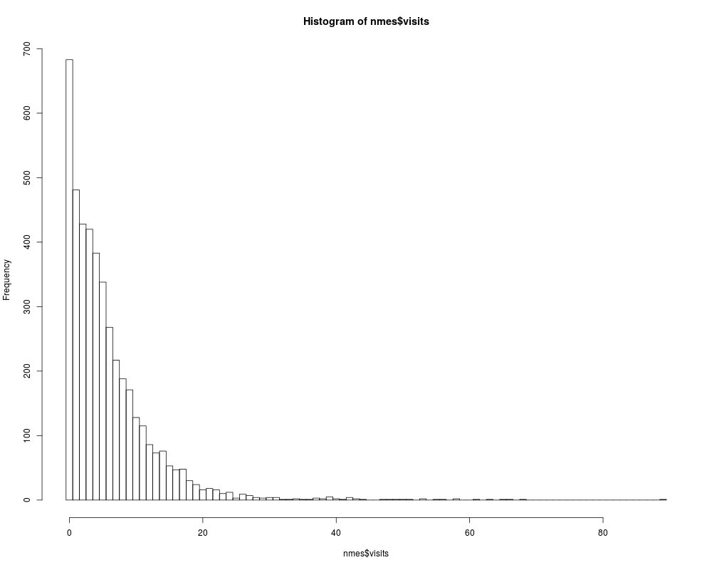
## dependent variable
hist(nmes$visits, breaks = 0:(max(nmes$visits)+1) - 0.5)
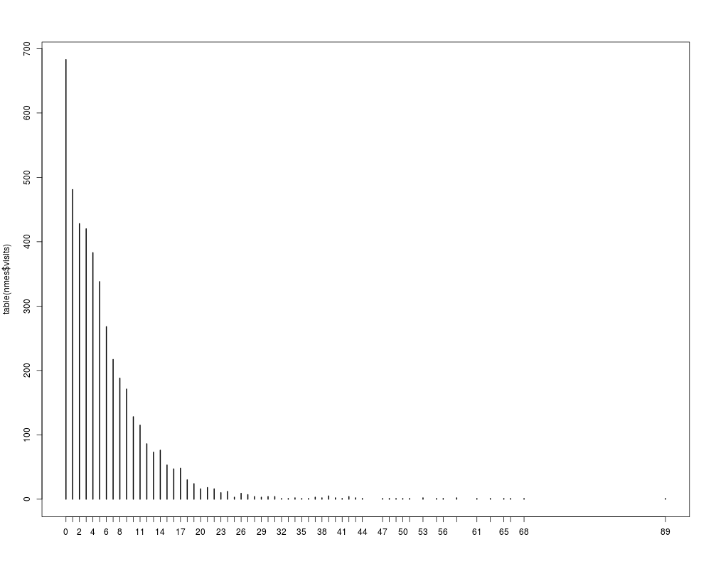
plot(table(nmes$visits))

## convenience transformations for exploratory graphics
clog <- function(x) log(x + 0.5)
cfac <- function(x, breaks = NULL) {
  if(is.null(breaks)) breaks <- unique(quantile(x, 0:10/10))
  x <- cut(x, breaks, include.lowest = TRUE, right = FALSE)
  levels(x) <- paste(breaks[-length(breaks)], ifelse(diff(breaks) > 1,
    c(paste("-", breaks[-c(1, length(breaks))] - 1, sep = ""), "+"), ""), sep = "")
  return(x)
}

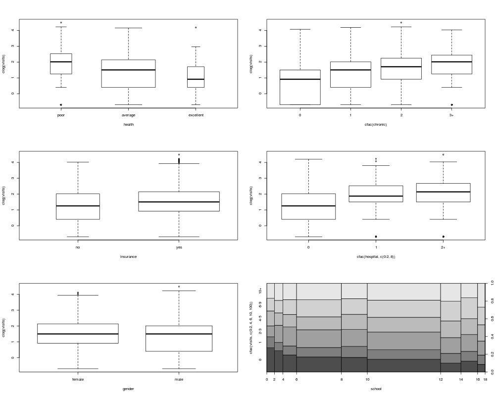
## bivariate visualization
par(mfrow = c(3, 2))
plot(clog(visits) ~ health, data = nmes, varwidth = TRUE)
plot(clog(visits) ~ cfac(chronic), data = nmes)
plot(clog(visits) ~ insurance, data = nmes, varwidth = TRUE)
plot(clog(visits) ~ cfac(hospital, c(0:2, 8)), data = nmes)
plot(clog(visits) ~ gender, data = nmes, varwidth = TRUE)
plot(cfac(visits, c(0:2, 4, 6, 10, 100)) ~ school, data = nmes, breaks = 9)
par(mfrow = c(1, 1))

## Poisson regression
nmes_pois <- glm(visits ~ ., data = nmes, family = poisson)
summary(nmes_pois)

## LM test for overdispersion
dispersiontest(nmes_pois)
dispersiontest(nmes_pois, trafo = 2)

## sandwich covariance matrix
coeftest(nmes_pois, vcov = sandwich)

## quasipoisson model
nmes_qpois <- glm(visits ~ ., data = nmes, family = quasipoisson)

## NegBin regression
nmes_nb <- glm.nb(visits ~ ., data = nmes)

## hurdle regression
nmes_hurdle <- hurdle(visits ~ . | hospital + chronic + insurance + school + gender,
  data = nmes, dist = "negbin")

## zero-inflated regression model
nmes_zinb <- zeroinfl(visits ~ . | hospital + chronic + insurance + school + gender,
  data = nmes, dist = "negbin")

## compare estimated coefficients
fm <- list("ML-Pois" = nmes_pois, "Quasi-Pois" = nmes_qpois, "NB" = nmes_nb,
  "Hurdle-NB" = nmes_hurdle, "ZINB" = nmes_zinb)
round(sapply(fm, function(x) coef(x)[1:8]), digits = 3)

## associated standard errors
round(cbind("ML-Pois" = sqrt(diag(vcov(nmes_pois))),
  "Adj-Pois" = sqrt(diag(sandwich(nmes_pois))),
  sapply(fm[-1], function(x) sqrt(diag(vcov(x)))[1:8])),
  digits = 3)

## log-likelihoods and number of estimated parameters
rbind(logLik = sapply(fm, function(x) round(logLik(x), digits = 0)),
  Df = sapply(fm, function(x) attr(logLik(x), "df")))

## predicted number of zeros
round(c("Obs" = sum(nmes$visits < 1),
  "ML-Pois" = sum(dpois(0, fitted(nmes_pois))),
  "Adj-Pois" = NA,
  "Quasi-Pois" = NA,
  "NB" = sum(dnbinom(0, mu = fitted(nmes_nb), size = nmes_nb$theta)),
  "NB-Hurdle" = sum(predict(nmes_hurdle, type = "prob")[,1]),
  "ZINB" = sum(predict(nmes_zinb, type = "prob")[,1])))

## coefficients of zero-augmentation models
t(sapply(fm[4:5], function(x) round(x$coefficients$zero, digits = 3)))

Results


R version 3.3.1 (2016-06-21) -- "Bug in Your Hair"
Copyright (C) 2016 The R Foundation for Statistical Computing
Platform: x86_64-pc-linux-gnu (64-bit)

R is free software and comes with ABSOLUTELY NO WARRANTY.
You are welcome to redistribute it under certain conditions.
Type 'license()' or 'licence()' for distribution details.

R is a collaborative project with many contributors.
Type 'contributors()' for more information and
'citation()' on how to cite R or R packages in publications.

Type 'demo()' for some demos, 'help()' for on-line help, or
'help.start()' for an HTML browser interface to help.
Type 'q()' to quit R.

> library(AER)
Loading required package: car
Loading required package: lmtest
Loading required package: zoo

Attaching package: 'zoo'

The following objects are masked from 'package:base':

    as.Date, as.Date.numeric

Loading required package: sandwich
Loading required package: survival
> png(filename="/home/ddbj/snapshot/RGM3/R_CC/result/AER/NMES1988.Rd_%03d_medium.png", width=480, height=480)
> ### Name: NMES1988
> ### Title: Demand for Medical Care in NMES 1988
> ### Aliases: NMES1988
> ### Keywords: datasets
> 
> ### ** Examples
> 
> ## packages
> library("MASS")
> library("pscl")
Loading required package: lattice
Classes and Methods for R developed in the

Political Science Computational Laboratory

Department of Political Science

Stanford University

Simon Jackman

hurdle and zeroinfl functions by Achim Zeileis

> 
> ## select variables for analysis
> data("NMES1988")
> nmes <- NMES1988[, c(1, 6:8, 13, 15, 18)]
> 
> ## dependent variable
> hist(nmes$visits, breaks = 0:(max(nmes$visits)+1) - 0.5)
> plot(table(nmes$visits))
> 
> ## convenience transformations for exploratory graphics
> clog <- function(x) log(x + 0.5)
> cfac <- function(x, breaks = NULL) {
+   if(is.null(breaks)) breaks <- unique(quantile(x, 0:10/10))
+   x <- cut(x, breaks, include.lowest = TRUE, right = FALSE)
+   levels(x) <- paste(breaks[-length(breaks)], ifelse(diff(breaks) > 1,
+     c(paste("-", breaks[-c(1, length(breaks))] - 1, sep = ""), "+"), ""), sep = "")
+   return(x)
+ }
> 
> ## bivariate visualization
> par(mfrow = c(3, 2))
> plot(clog(visits) ~ health, data = nmes, varwidth = TRUE)
> plot(clog(visits) ~ cfac(chronic), data = nmes)
> plot(clog(visits) ~ insurance, data = nmes, varwidth = TRUE)
> plot(clog(visits) ~ cfac(hospital, c(0:2, 8)), data = nmes)
> plot(clog(visits) ~ gender, data = nmes, varwidth = TRUE)
> plot(cfac(visits, c(0:2, 4, 6, 10, 100)) ~ school, data = nmes, breaks = 9)
> par(mfrow = c(1, 1))
> 
> ## Poisson regression
> nmes_pois <- glm(visits ~ ., data = nmes, family = poisson)
> summary(nmes_pois)

Call:
glm(formula = visits ~ ., family = poisson, data = nmes)

Deviance Residuals: 
    Min       1Q   Median       3Q      Max  
-8.4055  -1.9962  -0.6737   0.7049  16.3620  

Coefficients:
                 Estimate Std. Error z value Pr(>|z|)    
(Intercept)      1.028874   0.023785  43.258   <2e-16 ***
hospital         0.164797   0.005997  27.478   <2e-16 ***
healthpoor       0.248307   0.017845  13.915   <2e-16 ***
healthexcellent -0.361993   0.030304 -11.945   <2e-16 ***
chronic          0.146639   0.004580  32.020   <2e-16 ***
gendermale      -0.112320   0.012945  -8.677   <2e-16 ***
school           0.026143   0.001843  14.182   <2e-16 ***
insuranceyes     0.201687   0.016860  11.963   <2e-16 ***
---
Signif. codes:  0 '***' 0.001 '**' 0.01 '*' 0.05 '.' 0.1 ' ' 1

(Dispersion parameter for poisson family taken to be 1)

    Null deviance: 26943  on 4405  degrees of freedom
Residual deviance: 23168  on 4398  degrees of freedom
AIC: 35959

Number of Fisher Scoring iterations: 5

> 
> ## LM test for overdispersion
> dispersiontest(nmes_pois)

	Overdispersion test

data:  nmes_pois
z = 11.509, p-value < 2.2e-16
alternative hypothesis: true dispersion is greater than 1
sample estimates:
dispersion 
  6.706192 

> dispersiontest(nmes_pois, trafo = 2)

	Overdispersion test

data:  nmes_pois
z = 11.374, p-value < 2.2e-16
alternative hypothesis: true alpha is greater than 0
sample estimates:
    alpha 
0.8953912 

> 
> ## sandwich covariance matrix
> coeftest(nmes_pois, vcov = sandwich)

z test of coefficients:

                 Estimate Std. Error z value  Pr(>|z|)    
(Intercept)      1.028874   0.064530 15.9442 < 2.2e-16 ***
hospital         0.164797   0.021945  7.5095 5.935e-14 ***
healthpoor       0.248307   0.054022  4.5964 4.298e-06 ***
healthexcellent -0.361993   0.077449 -4.6740 2.954e-06 ***
chronic          0.146639   0.012908 11.3605 < 2.2e-16 ***
gendermale      -0.112320   0.035343 -3.1780  0.001483 ** 
school           0.026143   0.005084  5.1422 2.715e-07 ***
insuranceyes     0.201687   0.043128  4.6765 2.919e-06 ***
---
Signif. codes:  0 '***' 0.001 '**' 0.01 '*' 0.05 '.' 0.1 ' ' 1

> 
> ## quasipoisson model
> nmes_qpois <- glm(visits ~ ., data = nmes, family = quasipoisson)
> 
> ## NegBin regression
> nmes_nb <- glm.nb(visits ~ ., data = nmes)
> 
> ## hurdle regression
> nmes_hurdle <- hurdle(visits ~ . | hospital + chronic + insurance + school + gender,
+   data = nmes, dist = "negbin")
> 
> ## zero-inflated regression model
> nmes_zinb <- zeroinfl(visits ~ . | hospital + chronic + insurance + school + gender,
+   data = nmes, dist = "negbin")
> 
> ## compare estimated coefficients
> fm <- list("ML-Pois" = nmes_pois, "Quasi-Pois" = nmes_qpois, "NB" = nmes_nb,
+   "Hurdle-NB" = nmes_hurdle, "ZINB" = nmes_zinb)
> round(sapply(fm, function(x) coef(x)[1:8]), digits = 3)
                ML-Pois Quasi-Pois     NB Hurdle-NB   ZINB
(Intercept)       1.029      1.029  0.929     1.198  1.194
hospital          0.165      0.165  0.218     0.212  0.201
healthpoor        0.248      0.248  0.305     0.316  0.285
healthexcellent  -0.362     -0.362 -0.342    -0.332 -0.319
chronic           0.147      0.147  0.175     0.126  0.129
gendermale       -0.112     -0.112 -0.126    -0.068 -0.080
school            0.026      0.026  0.027     0.021  0.021
insuranceyes      0.202      0.202  0.224     0.100  0.126
> 
> ## associated standard errors
> round(cbind("ML-Pois" = sqrt(diag(vcov(nmes_pois))),
+   "Adj-Pois" = sqrt(diag(sandwich(nmes_pois))),
+   sapply(fm[-1], function(x) sqrt(diag(vcov(x)))[1:8])),
+   digits = 3)
                ML-Pois Adj-Pois Quasi-Pois    NB Hurdle-NB  ZINB
(Intercept)       0.024    0.065      0.062 0.055     0.059 0.057
hospital          0.006    0.022      0.016 0.020     0.021 0.020
healthpoor        0.018    0.054      0.046 0.049     0.048 0.045
healthexcellent   0.030    0.077      0.078 0.061     0.066 0.060
chronic           0.005    0.013      0.012 0.012     0.012 0.012
gendermale        0.013    0.035      0.034 0.031     0.032 0.031
school            0.002    0.005      0.005 0.004     0.005 0.004
insuranceyes      0.017    0.043      0.044 0.039     0.043 0.042
> 
> ## log-likelihoods and number of estimated parameters
> rbind(logLik = sapply(fm, function(x) round(logLik(x), digits = 0)),
+   Df = sapply(fm, function(x) attr(logLik(x), "df")))
       ML-Pois Quasi-Pois     NB Hurdle-NB   ZINB
logLik  -17972         NA -12171    -12090 -12091
Df           8          8      9        15     15
> 
> ## predicted number of zeros
> round(c("Obs" = sum(nmes$visits < 1),
+   "ML-Pois" = sum(dpois(0, fitted(nmes_pois))),
+   "Adj-Pois" = NA,
+   "Quasi-Pois" = NA,
+   "NB" = sum(dnbinom(0, mu = fitted(nmes_nb), size = nmes_nb$theta)),
+   "NB-Hurdle" = sum(predict(nmes_hurdle, type = "prob")[,1]),
+   "ZINB" = sum(predict(nmes_zinb, type = "prob")[,1])))
       Obs    ML-Pois   Adj-Pois Quasi-Pois         NB  NB-Hurdle       ZINB 
       683         47         NA         NA        608        683        709 
> 
> ## coefficients of zero-augmentation models
> t(sapply(fm[4:5], function(x) round(x$coefficients$zero, digits = 3)))
          (Intercept) hospital chronic insuranceyes school gendermale
Hurdle-NB       0.016    0.318   0.548        0.746  0.057     -0.419
ZINB           -0.047   -0.800  -1.248       -1.176 -0.084      0.648
> 
> 
> 
> 
> 
> dev.off()
null device 
          1 
>