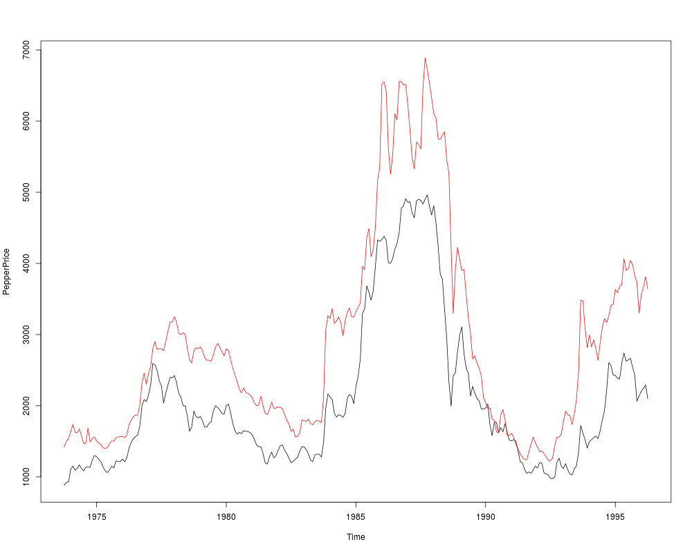
Black and White Pepper Prices

Description

Time series of average monthly European spot prices for black and white pepper (fair average quality) in US dollars per ton.

Usage

data("PepperPrice")

Format

A monthly multiple time series from 1973(10) to 1996(4) with 2 variables.

black

spot price for black pepper,

white

spot price for white pepper.

Source

Online complements to Franses (1998).

http://www.few.eur.nl/few/people/franses/research/book2.htm

References

Franses, P.H. (1998). Time Series Models for Business and Economic Forecasting. Cambridge, UK: Cambridge University Press.

Examples

## data
data("PepperPrice")
plot(PepperPrice, plot.type = "single", col = 1:2)

## package
library("tseries")
library("urca")

## unit root tests
adf.test(log(PepperPrice[, "white"]))
adf.test(diff(log(PepperPrice[, "white"])))
pp.test(log(PepperPrice[, "white"]), type = "Z(t_alpha)")
pepper_ers <- ur.ers(log(PepperPrice[, "white"]),
  type = "DF-GLS", model = "const", lag.max = 4)
summary(pepper_ers)

## stationarity tests
kpss.test(log(PepperPrice[, "white"]))

## cointegration
po.test(log(PepperPrice))
pepper_jo <- ca.jo(log(PepperPrice), ecdet = "const", type = "trace")
summary(pepper_jo)
pepper_jo2 <- ca.jo(log(PepperPrice), ecdet = "const", type = "eigen")
summary(pepper_jo2)

Results

R version 3.3.1 (2016-06-21) -- "Bug in Your Hair"
Copyright (C) 2016 The R Foundation for Statistical Computing
Platform: x86_64-pc-linux-gnu (64-bit)

R is free software and comes with ABSOLUTELY NO WARRANTY.
You are welcome to redistribute it under certain conditions.
Type 'license()' or 'licence()' for distribution details.

R is a collaborative project with many contributors.
Type 'contributors()' for more information and
'citation()' on how to cite R or R packages in publications.

Type 'demo()' for some demos, 'help()' for on-line help, or
'help.start()' for an HTML browser interface to help.
Type 'q()' to quit R.

> library(AER)
Loading required package: car
Loading required package: lmtest
Loading required package: zoo

Attaching package: 'zoo'

The following objects are masked from 'package:base':

    as.Date, as.Date.numeric

Loading required package: sandwich
Loading required package: survival
> png(filename="/home/ddbj/snapshot/RGM3/R_CC/result/AER/PepperPrice.Rd_%03d_medium.png", width=480, height=480)
> ### Name: PepperPrice
> ### Title: Black and White Pepper Prices
> ### Aliases: PepperPrice
> ### Keywords: datasets
> 
> ### ** Examples
> 
> ## data
> data("PepperPrice")
> plot(PepperPrice, plot.type = "single", col = 1:2)
> 
> ## package
> library("tseries")
> library("urca")
> 
> ## unit root tests
> adf.test(log(PepperPrice[, "white"]))

	Augmented Dickey-Fuller Test

data:  log(PepperPrice[, "white"])
Dickey-Fuller = -1.744, Lag order = 6, p-value = 0.6838
alternative hypothesis: stationary

> adf.test(diff(log(PepperPrice[, "white"])))

	Augmented Dickey-Fuller Test

data:  diff(log(PepperPrice[, "white"]))
Dickey-Fuller = -5.336, Lag order = 6, p-value = 0.01
alternative hypothesis: stationary

Warning message:
In adf.test(diff(log(PepperPrice[, "white"]))) :
  p-value smaller than printed p-value
> pp.test(log(PepperPrice[, "white"]), type = "Z(t_alpha)")

	Phillips-Perron Unit Root Test

data:  log(PepperPrice[, "white"])
Dickey-Fuller Z(t_alpha) = -1.6439, Truncation lag parameter = 5,
p-value = 0.726
alternative hypothesis: stationary

> pepper_ers <- ur.ers(log(PepperPrice[, "white"]),
+   type = "DF-GLS", model = "const", lag.max = 4)
> summary(pepper_ers)

############################################### 
# Elliot, Rothenberg and Stock Unit Root Test # 
############################################### 

Test of type DF-GLS 
detrending of series with intercept 


Call:
lm(formula = dfgls.form, data = data.dfgls)

Residuals:
     Min       1Q   Median       3Q      Max 
-0.21135 -0.03069 -0.00108  0.03030  0.31018 

Coefficients:
              Estimate Std. Error t value Pr(>|t|)    
yd.lag       -0.004022   0.006015  -0.669    0.504    
yd.diff.lag1  0.336267   0.061986   5.425 1.32e-07 ***
yd.diff.lag2 -0.105024   0.065414  -1.606    0.110    
yd.diff.lag3  0.001263   0.065366   0.019    0.985    
yd.diff.lag4  0.011251   0.062085   0.181    0.856    
---
Signif. codes:  0 '***' 0.001 '**' 0.01 '*' 0.05 '.' 0.1 ' ' 1

Residual standard error: 0.06481 on 261 degrees of freedom
Multiple R-squared:  0.1028,	Adjusted R-squared:  0.0856 
F-statistic:  5.98 on 5 and 261 DF,  p-value: 2.947e-05


Value of test-statistic is: -0.6686 

Critical values of DF-GLS are:
                 1pct  5pct 10pct
critical values -2.57 -1.94 -1.62

> 
> ## stationarity tests
> kpss.test(log(PepperPrice[, "white"]))

	KPSS Test for Level Stationarity

data:  log(PepperPrice[, "white"])
KPSS Level = 0.91295, Truncation lag parameter = 3, p-value = 0.01

Warning message:
In kpss.test(log(PepperPrice[, "white"])) :
  p-value smaller than printed p-value
> 
> ## cointegration
> po.test(log(PepperPrice))

	Phillips-Ouliaris Cointegration Test

data:  log(PepperPrice)
Phillips-Ouliaris demeaned = -24.099, Truncation lag parameter = 2,
p-value = 0.02404

> pepper_jo <- ca.jo(log(PepperPrice), ecdet = "const", type = "trace")
> summary(pepper_jo)

###################### 
# Johansen-Procedure # 
###################### 

Test type: trace statistic , without linear trend and constant in cointegration 

Eigenvalues (lambda):
[1] 4.931953e-02 1.350807e-02 2.081668e-17

Values of teststatistic and critical values of test:

          test 10pct  5pct  1pct
r <= 1 |  3.66  7.52  9.24 12.97
r = 0  | 17.26 17.85 19.96 24.60

Eigenvectors, normalised to first column:
(These are the cointegration relations)

           black.l2 white.l2   constant
black.l2  1.0000000  1.00000   1.000000
white.l2 -0.8892307 -5.09942   2.280911
constant -0.5569943 33.02742 -20.032441

Weights W:
(This is the loading matrix)

           black.l2    white.l2      constant
black.d -0.07472300 0.002453210 -4.958157e-18
white.d  0.02015611 0.003537005  8.850353e-18

> pepper_jo2 <- ca.jo(log(PepperPrice), ecdet = "const", type = "eigen")
> summary(pepper_jo2)

###################### 
# Johansen-Procedure # 
###################### 

Test type: maximal eigenvalue statistic (lambda max) , without linear trend and constant in cointegration 

Eigenvalues (lambda):
[1] 4.931953e-02 1.350807e-02 2.081668e-17

Values of teststatistic and critical values of test:

          test 10pct  5pct  1pct
r <= 1 |  3.66  7.52  9.24 12.97
r = 0  | 13.61 13.75 15.67 20.20

Eigenvectors, normalised to first column:
(These are the cointegration relations)

           black.l2 white.l2   constant
black.l2  1.0000000  1.00000   1.000000
white.l2 -0.8892307 -5.09942   2.280911
constant -0.5569943 33.02742 -20.032441

Weights W:
(This is the loading matrix)

           black.l2    white.l2      constant
black.d -0.07472300 0.002453210 -4.958157e-18
white.d  0.02015611 0.003537005  8.850353e-18

> 
> 
> 
> 
> 
> dev.off()
null device 
          1 
>